flowchart LR
    ZH["Z_H<br/>(settler mortality)"] --> XH["X_H<br/>(institutions 1800)"]
    XH --> XC["X_C<br/>(institutions today)"]
    XH --> AC["A_C<br/>(alternative channel:<br/>human capital, etc.)"]
    XC --> YC["Y_C<br/>(income today)"]
    AC --> YC
Historical Instruments and Contemporary Endogenous Regressors
Introduction
A lot of empirical work in development and growth economics relies on a particular kind of identification strategy: you find some historical event or variable that plausibly shifted an outcome you care about, and you use it as an instrument for a contemporary, endogenous regressor. The textbook example is Acemoglu, Johnson and Robinson (2001), who use settler mortality in the colonial period as an instrument for the quality of institutions today, in order to estimate the effect of institutions on current income per capita. The logic is that places where Europeans could not settle (high mortality) got extractive institutions, those institutions persisted, and so historical mortality is a source of as-good-as-random variation in institutions now.
This is a clever design, and there are by now dozens of papers built on the same template — a historical instrument for a contemporary endogenous variable. But there is a subtle problem with it that I think is underappreciated, and which Casey and Klemp (2021) lay out very cleanly.1 The issue is that there is a gap in time between when the instrument acts and when the endogenous variable is measured, and over that gap the historical variable can influence the present through channels other than the contemporary regressor you put on the right-hand side. When that happens, the conventional IV regression does not recover the structural parameter you think it does.
In this post I want to first build the intuition using the institutions example, then write down the slightly more general framework, and finally implement the resulting bias correction in both R (with fixest) and Python (with pyfixest), so we can see it actually work on simulated data.
The problem, intuitively
Stick with the institutions story. Let \(Z_H\) be settler mortality — the historical instrument, where the subscript \(H\) flags that it does its work in the historical period. Let \(X\) denote institutional quality, which is time-varying: \(X_H\) is institutions back in, say, 1800, and \(X_C\) is institutions in the contemporary period, say 1995. And let \(Y_C\) be contemporary income per capita.
The thing to keep in mind is that \(X_H\) is not observed. We do not have a clean measure of institutional quality in 1800; what we have is institutions now, \(X_C\). So when AJR run their regression, they instrument \(X_C\) with \(Z_H\).
Here is the worry. Settler mortality shifted institutions in 1800 (\(X_H\)). But 1800 institutions did not only affect today’s institutions (\(X_C\)). They very plausibly also affected lots of other things that carried forward to today and that themselves affect income — human capital, the structure of the economy, technology, culture. Call this bundle of other persistent channels \(A_C\), an “alternative channel”. If early institutions affect current income both through current institutions and through \(A_C\), then \(Z_H\) is correlated with the error term in a regression of \(Y_C\) on \(X_C\) alone. The exclusion restriction fails — not because \(Z_H\) is a bad instrument for \(X_H\), but because \(X_C\) is not the only way that \(X_H\) reaches \(Y_C\).
So what does the conventional IV estimate? That is the question the framework answers, and the answer turns out to be clean and interpretable.
The framework
Casey and Klemp write the data generating process as four equations. The first is the usual first stage: the instrument shifts historical institutions,
\[X_{H,i} = \psi Z_{H,i} + \varepsilon_{X_H,i}. \tag{1}\]
The second is persistence: historical institutions carry forward to the present, with a per-period persistence parameter \(\delta\),
\[X_{C,i} = \delta X_{H,i} + \varepsilon_{X_C,i}. \tag{2}\]
The third is the alternative channel: historical institutions also shape some other contemporary variable \(A_C\) (unobserved), with strength \(\gamma\),
\[A_{C,i} = \gamma X_{H,i} + \varepsilon_{A,i}. \tag{3}\]
And the fourth is the outcome equation: contemporary income depends on both contemporary institutions and the alternative channel,
\[Y_{C,i} = \beta_1 X_{C,i} + \beta_2 A_{C,i} + \varepsilon_{Y,i}. \tag{4}\]
The maintained assumption is that the instrument is exogenous in the right sense: \(Z_H\) is uncorrelated with the structural errors \(\varepsilon_{X_C}\), \(\varepsilon_A\) and \(\varepsilon_Y\). Crucially, this does not say that \(Z_H\) is excludable from the \(Y_C\)-on-\(X_C\) regression — it isn’t, precisely because of the \(A_C\) channel.
Now, what is the parameter of interest? In a purely contemporaneous world you would want \(\beta_1\), the effect of today’s institutions on today’s income. But once you take the historical design seriously, the natural object is the long-run effect of historical institutions on current income,
\[\eta \equiv \frac{\partial Y_C}{\partial X_H}.\]
Substituting (2) and (3) into (4) gives \(Y_{C,i} = (\delta\beta_1 + \beta_2\gamma)X_{H,i} + \mu_i\), so
\[\eta = \delta\beta_1 + \beta_2\gamma.\]
The long-run effect is the sum of the part that runs through institutions (\(\delta\beta_1\)) and the part that runs through everything else (\(\beta_2\gamma\)).
What conventional IV actually estimates
Now run the conventional 2SLS: regress \(Y_C\) on \(X_C\), instrumenting with \(Z_H\). A few lines of covariance algebra (this is equation (9) in the paper) give
\[\text{plim}\,\hat{b}_1^{IV} = \beta_1 + \frac{\beta_2\gamma}{\delta} = \frac{\eta}{\delta}.\]
This is the key result, and it is worth pausing on. The conventional IV coefficient is neither \(\beta_1\) nor \(\eta\). It is the long-run effect \(\eta\) divided by the persistence \(\delta\).
The two coincide only in the knife-edge case \(\delta = 1\), i.e. perfect persistence. Whenever institutions are imperfectly persistent — \(\delta < 1\), which is surely the empirically relevant case — the conventional IV overstates the long-run effect, because you are dividing by a number less than one. Intuitively, \(X_C\) is a noisy, attenuated proxy for the thing the instrument actually shocked, \(X_H\), and the degree of attenuation is exactly \(\delta\). Casey and Klemp frame this nicely as a form of non-classical measurement error: we want the effect of \(X_H\), but we are forced to use a mismeasured version of it, \(X_C\), with the measurement error governed by how much of the original shock has decayed. A large IV coefficient might mean institutions matter a lot — or it might just mean institutions are not very persistent.
Recovering the long-run effect
The reason the conventional regression can’t be fixed by itself is that the single regression \(\hat b_1^{IV} = \eta/\delta\) has two structural unknowns in it, \(\eta\) and \(\delta\), and one equation. We need a second moment to separate them, and the natural one is an estimate of persistence \(\delta\).
The trouble is that \(\delta\) relates \(X_C\) to the unobserved \(X_H\), so we can’t estimate it directly. Casey and Klemp’s solution is to use the endogenous variable measured at two intermediate points in time — institutions are, after all, something we can measure historically with datasets like Polity. Suppose we observe \(X\) at periods \(T-Q\) and \(T\) (e.g. 1900 and 1965). Persistence compounds, so regressing \(X_T\) on \(X_{T-Q}\) — again instrumenting with \(Z_H\) to clean out measurement error — recovers
\[\text{plim}\,\hat{a}_1 = \delta^{Q},\]
the persistence of institutions over those \(Q\) periods. Raising this to the power \((C-H)/Q\) extrapolates it to persistence over the full historical-to-contemporary gap, \(\delta^{C-H}\). Multiplying the conventional IV coefficient by this factor cancels the division and recovers the long-run effect:
\[\eta = \big(\text{plim}\,\hat{b}_1^{IV}\big)\cdot\big(\text{plim}\,\hat{a}_1\big)^{\frac{C-H}{Q}} = \frac{\eta}{\delta^{C-H}}\cdot\delta^{C-H}.\]
In words: run two IV regressions — the conventional one for \(\eta/\delta^{C-H}\), and a persistence regression for \(\delta^{Q}\) — and combine them. The two are estimated jointly so that standard errors (via the delta method, or as I’ll do below, a bootstrap) account for the fact that both come from the same data. This rests on two assumptions worth flagging: that persistence \(\delta\) is roughly constant over time and that the law of motion is linear. Both are testable when you have panel data on the endogenous variable, and the paper spends a good deal of effort validating them for institutions.
What this does to the institutions result
When Casey and Klemp apply this to AJR, the correction bites hard. Institutions are persistent but far from perfectly so — their estimate of persistence over 1900–1965 is around \(0.69\), which extrapolated over the full 1800–1995 gap implies that only about a third of an initial institutional shock survives to the present. Running the correction, an improvement in Constraints on the Executive from the lowest to the highest score in 1800 raises 1990s income per capita by roughly \(0.85\) standard deviations — economically large, but only about one-third the size implied by the conventional IV coefficient. The headline qualitative finding survives; the magnitude does not.
Simulating it
The cleanest way to convince yourself of all this is to simulate data from equations (1)–(4), where we know the true \(\eta\), and check that (i) the conventional IV overshoots by the factor \(1/\delta^{C-H}\) and (ii) the two-step correction recovers the truth.
I’ll use the following design throughout. Settler mortality \(Z\sim N(0,1)\); historical institutions \(X_H = \psi Z + \varepsilon\); institutions decay with a per-year persistence factor \(d = 0.9943\), observed at 1900, 1965 and 1995; an unobserved channel \(A_C = \gamma X_H + \varepsilon\); and income \(Y_C = \beta_1 X_C + \beta_2 A_C + \varepsilon\), with \(\psi=1\), \(\beta_1=0.3\), \(\beta_2=0.4\) and \(\gamma=0.1\). These numbers are picked so the example mirrors the paper: the true long-run effect is \(\eta = \beta_1 d^{195} + \beta_2\gamma \approx 0.14\), persistence over 1900–1965 is \(d^{65}\approx 0.69\), and so the conventional IV should land near \(\eta/d^{195}\approx 0.42\) — about three times too big.
In R, with fixest
fixest’s feols takes IV specifications with the syntax y ~ exog | endog ~ instrument, which makes both of our regressions one-liners. First the data-generating process and the implied population truths:
library(fixest)
library(ggplot2)

# Casey & Klemp (2021) DGP. A historical instrument Z acts on institutions in
# period H (1800). Institutions persist at rate `d` per year and are observed at
# 1900, 1965 (to estimate persistence) and 1995 (the contemporary regressor).
simulate_ck <- function(N, seed = NULL) {
  if (!is.null(seed)) set.seed(seed)

  H <- 1800; t1 <- 1900; t2 <- 1965; C <- 1995
  d <- 0.9943                                   # per-year persistence
  psi <- 1; b1 <- 0.3; b2 <- 0.4; gamma <- 0.1
  sigma <- 0.3

  Z      <- rnorm(N, 0, 1)                       # historical instrument (settler mortality)
  X_H    <- psi * Z + rnorm(N, 0, sigma)         # historical institutions (1800), UNOBSERVED
  X_1900 <- d^(t1 - H) * X_H + rnorm(N, 0, sigma)
  X_1965 <- d^(t2 - H) * X_H + rnorm(N, 0, sigma)
  X_C    <- d^(C  - H) * X_H + rnorm(N, 0, sigma) # contemporary institutions (1995)
  A_C    <- gamma * X_H + rnorm(N, 0, sigma)      # unobserved alternative channel
  Y_C    <- b1 * X_C + b2 * A_C + rnorm(N, 0, sigma) # contemporary income

  data.frame(Z, X_1900, X_1965, X_C, Y_C)
}

# Implied population truths
d          <- 0.9943; b1 <- 0.3; b2 <- 0.4; gamma <- 0.1
eta_true    <- b1 * d^195 + b2 * gamma          # long-run structural effect (~0.138)
conv_target <- eta_true / d^195                 # conventional-IV probability limit (~0.422)
a1_target   <- d^65                             # 65-year persistence (~0.690)
corr_exp    <- (1995 - 1800) / (1965 - 1900)    # correction exponent = 195/65 = 3
Now draw one large sample and run the two IV regressions — the conventional one and the persistence one:
df <- simulate_ck(N = 2000, seed = 42)

# Conventional IV: instrument contemporary institutions with the historical Z.
# fixest names the fitted endogenous regressor `fit_X_C`.
iv_conv <- feols(Y_C ~ 1 | X_C ~ Z, data = df)
b_iv    <- coef(iv_conv)["fit_X_C"]              # ~0.42, the biased long-run effect

# Persistence IV: estimate delta^65 from two intermediate observations of X,
# again instrumenting with Z to purge measurement error.
iv_pers <- feols(X_1965 ~ 1 | X_1900 ~ Z, data = df)
a1      <- coef(iv_pers)["fit_X_1900"]           # ~0.69

# Bias-corrected long-run effect: scale the conventional IV back by persistence.
eta_hat <- unname(b_iv * a1^corr_exp)            # ~0.14
A pairs bootstrap gives a standard error that accounts for both regressions being estimated on the same data:
boot_eta <- function(data, reps = 1000, seed = 2021) {
  set.seed(seed)
  n <- nrow(data)
  out <- numeric(reps)
  for (r in seq_len(reps)) {
    bd <- data[sample.int(n, n, replace = TRUE), ]   # resample units with replacement
    bi <- coef(feols(Y_C    ~ 1 | X_C    ~ Z, data = bd))["fit_X_C"]
    ai <- coef(feols(X_1965 ~ 1 | X_1900 ~ Z, data = bd))["fit_X_1900"]
    out[r] <- bi * ai^corr_exp
  }
  out
}

eta_boot <- boot_eta(df, reps = 1000)
eta_se   <- sd(eta_boot)
comparison <- data.frame(
quantity = c("True eta (long-run effect)",
"Conventional IV (= eta / delta^195)",
"Persistence a1 (= delta^65)",
"Bias-corrected eta_hat"),
target = c(eta_true, conv_target, a1_target, eta_true),
estimate = c(NA, b_iv, a1, eta_hat),
boot_se = c(NA, NA, NA, eta_se)
)
print(comparison, row.names = FALSE, digits = 4) quantity target estimate boot_se
True eta (long-run effect) 0.1384 NA NA
Conventional IV (= eta / delta^195) 0.4219 0.4221 NA
Persistence a1 (= delta^65) 0.6897 0.6908 NA
Bias-corrected eta_hat 0.1384 0.1391 0.01176The conventional IV coefficient is about \(0.42\), three times the true long-run effect, exactly as the formula \(\eta/\delta^{195}\) predicts; the corrected estimate is \(\approx 0.14\), essentially equal to the true \(\eta\). To see this is not a fluke of one sample, a Monte Carlo over paper-sized samples (\(N=200\)):
run_mc <- function(reps = 1000, N = 200, seed = 7) {
  set.seed(seed)
  conv <- corr <- numeric(reps)
  for (r in seq_len(reps)) {
    d_r <- simulate_ck(N)
    bi  <- coef(feols(Y_C    ~ 1 | X_C    ~ Z, data = d_r))["fit_X_C"]
    ai  <- coef(feols(X_1965 ~ 1 | X_1900 ~ Z, data = d_r))["fit_X_1900"]
    conv[r] <- bi
    corr[r] <- bi * ai^corr_exp
  }
  rbind(
    data.frame(estimator = "Conventional IV", value = conv),
    data.frame(estimator = "Bias-corrected",  value = corr)
  )
}

mc <- run_mc(reps = 1000, N = 200, seed = 7)   # smaller, paper-like sample

ggplot(mc, aes(x = value, fill = estimator)) +
  geom_density(alpha = 0.45, color = NA) +
  geom_vline(xintercept = eta_true, linetype = "dashed") +
  annotate("text", x = eta_true, y = 0, label = "  true eta",
           hjust = 0, vjust = -0.5, size = 3) +
  labs(x = "Estimated effect", y = "Density", fill = NULL,
       title = "Conventional IV vs. bias-corrected long-run effect",
       subtitle = "1000 Monte Carlo replications, N = 200") +
  theme_minimal()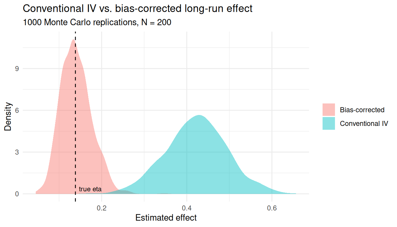
The conventional estimator’s density sits over \(0.42\) while the bias-corrected one is centered on the dashed line at the true \(\eta\) — the same picture we’ll get in Python.
In Python, with pyfixest
The same exercise translates directly. pyfixest mirrors fixest’s formula interface, including the Y ~ 1 | X ~ Z IV syntax, so the code reads almost identically. We start with the parameters and a function that draws one cross-section from the DGP:
import numpy as np
import pandas as pd
import pyfixest as pf
import matplotlib.pyplot as plt

# DGP parameters --------------------------------------------------------------
H, C   = 1800, 1995        # historical / contemporary periods
T1, T2 = 1900, 1965        # two intermediate observations of institutions
d      = 0.9943            # per-year persistence of institutions
psi, b1, b2, gamma = 1.0, 0.3, 0.4, 0.1
sigma  = 0.3               # sd of all iid N(0, sigma) errors

# Implied structural quantities
eta         = b1 * d ** (C - H) + b2 * gamma   # true long-run effect  ~ 0.1385
conv_target = eta / d ** (C - H)               # conventional-IV target ~ 0.422
a1_target   = d ** (T2 - T1)                    # persistence-IV target  ~ 0.690
expo        = (C - H) / (T2 - T1)               # correction exponent = 195/65 = 3
def simulate(n, rng):
"""One cross-section of n units following the Casey & Klemp (2021) DGP."""
Z = rng.normal(0, 1, n) # instrument (settler mortality)
X_H = psi * Z + rng.normal(0, sigma, n) # 1800 institutions, UNOBSERVED
X_1900 = d ** (T1 - H) * X_H + rng.normal(0, sigma, n) # observed
X_1965 = d ** (T2 - H) * X_H + rng.normal(0, sigma, n) # observed
X_C = d ** (C - H) * X_H + rng.normal(0, sigma, n) # 1995 institutions, observed
A_C = gamma * X_H + rng.normal(0, sigma, n) # alternative channel, UNOBSERVED
Y_C = b1 * X_C + b2 * A_C + rng.normal(0, sigma, n) # contemporary income, observed
return pd.DataFrame(
{"Z": Z, "X_1900": X_1900, "X_1965": X_1965, "X_C": X_C, "Y_C": Y_C}
)
def estimates(df):
"""Conventional IV coef, persistence a1, and bias-corrected eta_hat."""
# Conventional 2SLS: instrument contemporary institutions X_C with Z.
b_iv = pf.feols("Y_C ~ 1 | X_C ~ Z", data=df).coef()["X_C"]
# Persistence regression: instrument X_1900 with Z to recover per-period decay.
a1 = pf.feols("X_1965 ~ 1 | X_1900 ~ Z", data=df).coef()["X_1900"]
# Multiply by a1 raised to the inter-period correction exponent.
eta_hat = b_iv * a1 ** expo
return b_iv, a1, eta_hatOne large sample gives the three numbers:
rng = np.random.default_rng(20210)
df  = simulate(2000, rng)

b_iv, a1, eta_hat = estimates(df)
b_iv, a1, eta_hat   # ~0.41, ~0.69, ~0.13
(np.float64(0.4122985605179479), np.float64(0.6874282441344046), np.float64(0.1339349544022558))A pairs bootstrap gives a standard error for the corrected estimate that respects the fact that both regressions come from the same data:
# Pairs bootstrap: resample units with replacement, refit both models, recompute eta_hat.
B = 1000
boot = np.empty(B)
for b in range(B):
    idx = rng.integers(0, len(df), len(df))
    boot[b] = estimates(df.iloc[idx].reset_index(drop=True))[2]
eta_se = boot.std(ddof=1)
eta_senp.float64(0.010899121177414947)summary = pd.DataFrame(
{
"quantity": [
"true eta",
"conventional IV (eta/delta^195)",
"persistence a1 (delta^65)",
"bias-corrected eta_hat",
],
"target": [eta, conv_target, a1_target, eta],
"estimate": [np.nan, b_iv, a1, eta_hat],
"boot_se": [np.nan, np.nan, np.nan, eta_se],
}
)
summary quantity target estimate boot_se
0 true eta 0.138406 NaN NaN
1 conventional IV (eta/delta^195) 0.421944 0.412299 NaN
2 persistence a1 (delta^65) 0.689658 0.687428 NaN
3 bias-corrected eta_hat 0.138406 0.133935 0.010899The conventional IV lands near \(0.41\) — about three times the true long-run effect — exactly because it estimates \(\eta/\delta^{195}\). Multiplying by the separately-estimated persistence \(\hat a_1^{3}\) brings it back to \(\eta\approx 0.13\). Finally, a Monte Carlo over paper-sized samples (\(N=200\)) shows the two sampling distributions side by side:
# Paper-like small samples: contrast the two sampling distributions.
R, n_mc = 1000, 200
mc_iv, mc_eta = np.empty(R), np.empty(R)
mc_rng = np.random.default_rng(7)
for r in range(R):
    b, _, e = estimates(simulate(n_mc, mc_rng))
    mc_iv[r], mc_eta[r] = b, e

fig, ax = plt.subplots(figsize=(8, 5))
ax.hist(mc_iv,  bins=40, alpha=0.6, label="Conventional IV", color="#c1121f")
(array([ 1., 2., 0., 1., 2., 0., 4., 12., 13., 11., 30., 27., 42.,
51., 57., 55., 54., 68., 68., 57., 68., 61., 59., 61., 42., 30.,
30., 24., 18., 12., 10., 7., 8., 5., 4., 3., 1., 0., 1.,
1.]), array([0.19978963, 0.21153716, 0.22328469, 0.23503222, 0.24677975,
0.25852728, 0.27027482, 0.28202235, 0.29376988, 0.30551741,
0.31726494, 0.32901247, 0.34076 , 0.35250754, 0.36425507,
0.3760026 , 0.38775013, 0.39949766, 0.41124519, 0.42299272,
0.43474026, 0.44648779, 0.45823532, 0.46998285, 0.48173038,
0.49347791, 0.50522544, 0.51697298, 0.52872051, 0.54046804,
0.55221557, 0.5639631 , 0.57571063, 0.58745816, 0.5992057 ,
0.61095323, 0.62270076, 0.63444829, 0.64619582, 0.65794335,
0.66969088]), <BarContainer object of 40 artists>)ax.hist(mc_eta, bins=40, alpha=0.6, label=r"Bias-corrected $\hat\eta$", color="#386641")(array([ 2., 3., 5., 7., 18., 41., 30., 44., 55., 82., 68., 67., 76.,
60., 51., 62., 63., 38., 43., 34., 19., 29., 17., 13., 14., 15.,
9., 4., 9., 5., 5., 7., 2., 2., 0., 0., 0., 0., 0.,
1.]), array([0.05761625, 0.06364365, 0.06967106, 0.07569847, 0.08172587,
0.08775328, 0.09378069, 0.0998081 , 0.1058355 , 0.11186291,
0.11789032, 0.12391773, 0.12994513, 0.13597254, 0.14199995,
0.14802736, 0.15405476, 0.16008217, 0.16610958, 0.17213699,
0.17816439, 0.1841918 , 0.19021921, 0.19624662, 0.20227402,
0.20830143, 0.21432884, 0.22035625, 0.22638365, 0.23241106,
0.23843847, 0.24446588, 0.25049328, 0.25652069, 0.2625481 ,
0.2685755 , 0.27460291, 0.28063032, 0.28665773, 0.29268513,
0.29871254]), <BarContainer object of 40 artists>)ax.axvline(eta, ls="--", color="black", lw=1.5, label=fr"True $\eta$ = {eta:.3f}")<matplotlib.lines.Line2D object at 0x7f198d6c8400>ax.set_xlabel("Estimate")Text(0.5, 0, 'Estimate')ax.set_ylabel("Frequency")Text(0, 0.5, 'Frequency')ax.set_title("Sampling distributions (N = 200, 1000 reps)")Text(0.5, 1.0, 'Sampling distributions (N = 200, 1000 reps)')ax.legend()<matplotlib.legend.Legend object at 0x7f198d7a7b20>fig.tight_layout()
plt.show()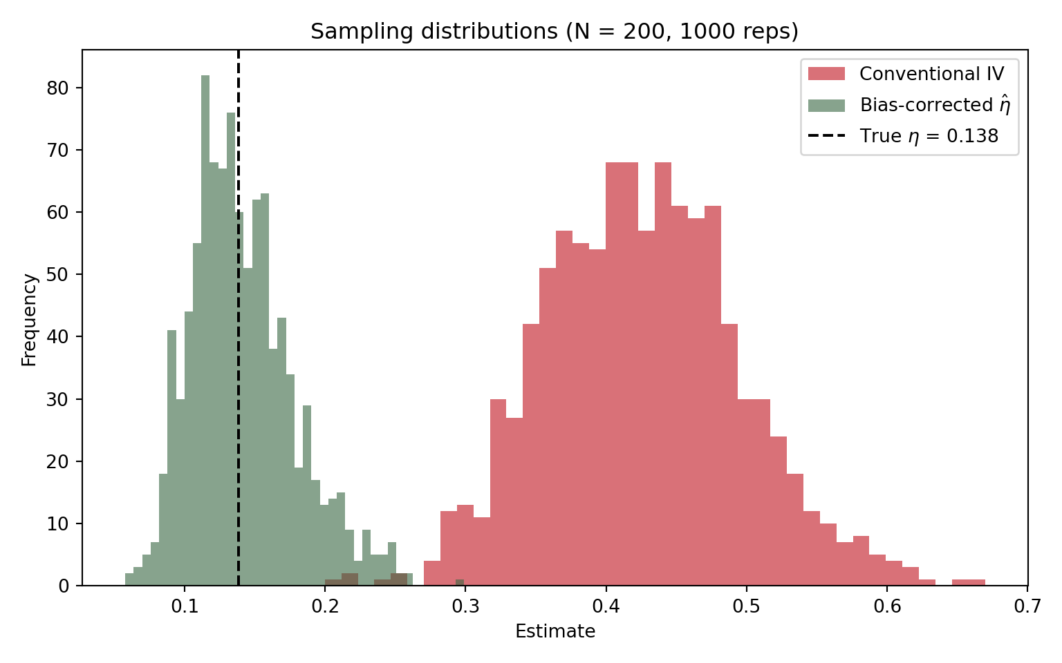
The conventional IV is centered well to the right of the truth; the corrected estimator sits right on top of the dashed line at \(\eta\).
Closing thoughts
What I like about this paper is that it takes a research design everyone uses and shows, with very little machinery, that the coefficient it produces has a specific and somewhat awkward interpretation: not the contemporaneous effect, not the long-run effect, but their ratio with persistence. That is the kind of result that is obvious only in hindsight. The practical advice is also reassuring rather than nihilistic — if you have the endogenous variable measured at a couple of historical dates, you can separately estimate persistence and back out the long-run effect; and even when you can’t, the reduced-form and first-stage regressions still tell you whether a long-run channel exists and what sign it has, which is often what you actually wanted to know.
I hope this has been a useful walk-through. If you spot an error or have suggestions, let me know, and thanks for reading.
Footnotes
Casey, G., & Klemp, M. (2021). Historical instruments and contemporary endogenous regressors. Journal of Development Economics, 149, 102586.↩︎