Who Moves to the City? Estimating the Roy Model of Selection
Author
Bas Machielsen
Published
May 10, 2026
Introduction
Suppose you want to know whether migrants earned more than stayers. You have census data: wages for people observed in the city and wages for people observed in the countryside. The difference in means tells you something, but not what you want. The people who moved are not a random draw. They moved because they expected to gain from it, and that expectation is correlated with what they would have earned had they stayed. The naive comparison is contaminated by selection, and the sign of the contamination is not obvious. Migrants might be positively selected (the most able move) or negatively selected (those with the least to lose move), and which it is changes the answer.
This is the problem the Roy model solves. It gives you a framework in which the selection is part of the model rather than a nuisance to be swept away. You write down the choice, you write down the potential outcomes, and you estimate the whole thing together. By the end you can answer the counterfactual: what would the migrant have earned at home?
The model originates with Roy (1951), who was thinking about hunters and fishermen,1 and it was developed econometrically by Heckman (1979)2 and Lee (1978).3 Borjas (1987) applied it to the earnings of immigrants,4 and economic historians have used it to study migration (Abramitzky, Boustan, and Eriksson 2012 on the age of mass migration),5 occupational choice, and sectoral reallocation during industrialization. This post walks through the model, the estimation, and a full implementation in Python, using rural-to-urban migration in a nineteenth-century setting as the running example.
The Model
An individual \(i\) faces two sectors: rural (0) and urban (1). In each sector they would earn a log wage
where \(\mathbf{x}_i\) is a vector of observable characteristics: age, literacy, whether their father was a farmer; and the coefficients can differ across sectors. Literacy might be worth more in the city than in the countryside; the model lets the data tell you.
The individual chooses the city if the gain exceeds the cost of moving:
\[
I_i^* = y_{1i} - y_{0i} - C_i,
\]
where \(C_i\) is a migration cost. Write the cost as \(C_i = \mathbf{z}_i \boldsymbol{\gamma} + u_i\), where \(\mathbf{z}_i\) contains variables that shift the cost but do not directly enter the wage equations. The canonical instrument in the migration literature is a network variable: does the individual have a sibling or a former neighbour already in the city? That makes moving cheaper: you have a place to stay, someone to vouch for you, without making you a more productive worker once you arrive.
We observe \((\mathbf{x}_i, \mathbf{z}_i, I_i, y_i)\); we do not observe the counterfactual wage.
The model is structural because the selection equation is not an afterthought. It comes from the same potential outcomes that generate the wages. The error term \(\eta_i\) contains \(\varepsilon_{1i} - \varepsilon_{0i}\), so the choice of sector is the comparative advantage. People who would earn unusually much in the city relative to the countryside are the ones who move. That is the economics; the econometrics just takes it seriously.
with \(\eta_i\) normalized to unit variance because the scale of \(I_i^*\) is not identified from a binary choice. The covariances \(\sigma_{0\eta}\) and \(\sigma_{1\eta}\) capture the selection. If \(\sigma_{1\eta} > 0\), people with high urban wage potential are more likely to move: positive selection into the city. If \(\sigma_{0\eta} < 0\), people with high rural wage potential are less likely to leave: negative selection out of the countryside. Both can operate at once.
Why Naive OLS Fails
Before estimating the structural model, it is worth seeing exactly how selection contaminates the naive comparison. I will work through the derivation in full because it is the central piece of machinery in every selection model.
Start with the wage equation for the urban sector:
The event \(I_i = 1\) is equivalent to \(I_i^* > 0\), which is \(\eta_i > -\mathbf{w}_i\boldsymbol{\delta}\). So the term we need is \(E[\varepsilon_{1i} \mid \eta_i > -\mathbf{w}_i\boldsymbol{\delta}]\), and it is not zero unless \(\varepsilon_{1i}\) and \(\eta_i\) are uncorrelated. We need to evaluate it under the joint normality assumption.
Step 1: The conditional mean of a bivariate normal
Take any two jointly normal random variables \((X, Y)\) with means \(\mu_X, \mu_Y\), variances \(\sigma^2_X, \sigma^2_Y\), and covariance \(\sigma_{XY}\). The conditional distribution of \(Y\) given \(X\) is normal with mean
This is the linear projection of \(Y\) on \(X\), and under joint normality it is exact. Apply it to \(X = \eta_i\) and \(Y = \varepsilon_{1i}\). Both have mean zero, \(\mathrm{Var}(\eta_i) = 1\), and \(\mathrm{Cov}(\varepsilon_{1i}, \eta_i) = \sigma_{1\eta}\), so
where \(c \equiv -\mathbf{w}_i\boldsymbol{\delta}\) for brevity.
Step 3: The mean of a truncated standard normal
The last piece is the expected value of a standard normal random variable when we only observe it above a threshold \(c\). For \(\eta_i \sim \mathcal{N}(0, 1)\),
where \(\phi(\cdot)\) is the standard normal density and \(\Phi(\cdot)\) is the standard normal cumulative distribution function. This ratio is the inverse Mills ratio, denoted \(\lambda(c)\). It is always positive: for \(c = 0\) it equals \(\sqrt{2/\pi} \approx 0.80\), it rises as \(c\) increases (a more selective threshold yields a higher mean among those who clear it), and it falls toward zero as \(c \to -\infty\) (when almost everyone passes, the truncation barely bites).
The OLS regression on the urban subsample omits \(\lambda(-\mathbf{w}_i\boldsymbol{\delta})\), and because \(\mathbf{x}_i\) appears in the selection equation through \(\mathbf{w}_i\boldsymbol{\delta}\), the omitted term is correlated with the included regressors. The OLS estimator of \(\boldsymbol{\beta}_1\) is therefore biased and inconsistent. The sign of the bias is the sign of \(\sigma_{1\eta}\) multiplied by the partial correlation between \(\mathbf{x}_i\) and the Mills ratio, which is typically positive: people with higher \(x\)’s are more likely to select into the urban sector, so \(x\) and \(\lambda\) covary positively, and if \(\sigma_{1\eta} > 0\) the OLS coefficients are inflated.
The rural side
The same logic applies to the rural sample, except the conditioning event is \(\eta_i \le -\mathbf{w}_i\boldsymbol{\delta}\). For a standard normal truncated from above at \(c\),
This is more than a technical footnote. If the most able rural workers are the ones who migrate (plausibly true), then \(\sigma_{1\eta} > 0\) and naive OLS overstates urban returns to ability. The model corrects for that.
Estimation
There are two standard approaches. The two-step method (Heckman 1979) is transparent and easy to implement. Full-information maximum likelihood (FIML) is more efficient but requires numerical optimization. I’ll show both.
Two-Step Estimation
Step 1. Estimate a probit of \(I_i\) on \(\mathbf{w}_i\) to get \(\hat{\boldsymbol{\delta}}\). Construct the inverse Mills ratios:
The coefficients on the Mills ratios estimate \(\sigma_{1\eta}\) and \(\sigma_{0\eta}\). If they are significantly different from zero, selection is present. Their signs tell you the direction: \(\hat{\theta}_1 > 0\) means positive selection into the urban sector.
The standard errors from the second-step OLS are wrong (the Mills ratio is a generated regressor), but you can bootstrap or use the analytical correction. In the code below I bootstrap.
Full-Information Maximum Likelihood
The likelihood for an individual with \(I_i = 1\) and observed wage \(y_i\) is
where \(f(y_i \mid I_i = 1)\) is the conditional density of the urban wage given selection. Under joint normality this density has a known form, and the joint likelihood across both regimes is
You maximize the log of this over all parameters simultaneously. The advantage is efficiency and coherent standard errors. The cost is that the likelihood can be flat in some directions, especially the correlation parameters, so you need reasonable starting values, which the two-step estimator helpfully provides.
Implementation in Python
I’ll simulate a dataset that mirrors the structure of nineteenth-century migration: roughly 15–20 percent of the population moves to the city; literacy and age shift wages in both sectors but literacy is valued more in the urban sector; and having a family connection in the city lowers the cost of moving.
import numpy as npimport pandas as pdfrom scipy.stats import norm, multivariate_normalfrom scipy.optimize import minimizeimport statsmodels.api as smimport matplotlib.pyplot as plt# ---- set seed and parameters ----np.random.seed(1848)N =4000# true parametersbeta0 = np.array([2.0, 0.06, 0.12]) # rural: intercept, age, literacybeta1 = np.array([2.2, 0.08, 0.35]) # urban: intercept, age, literacygamma = np.array([0.8, -1.2]) # cost: intercept, networksigma0 =0.55sigma1 =0.65rho_0eta =-0.45# selection: rural wage ↔ migrationrho_1eta =0.55# selection: urban wage ↔ migration# ---- simulate data ----age = np.random.normal(35, 12, N)literacy = np.random.binomial(1, 0.55, N)X = np.column_stack([np.ones(N), age, literacy])# network: family in the city (instrument)network = np.random.binomial(1, 0.25, N)# joint errors: (eps0, eps1, eta) where eta is the unobserved net cost of movingcov_matrix = np.array([ [sigma0**2, 0, rho_0eta * sigma0], [0, sigma1**2, rho_1eta * sigma1], [rho_0eta * sigma0, rho_1eta * sigma1, 1.0]])eps0, eps1, eta = multivariate_normal.rvs(cov=cov_matrix, size=N).T# potential wagesy0 = X @ beta0 + eps0y1 = X @ beta1 + eps1# selection: I* = X(beta1-beta0) - cost + eta# cost = gamma0 + gamma1 * network (higher with no network, lower with one)I_star = X @ (beta1 - beta0) - (gamma[0] + gamma[1] * network) + etamigrate = (I_star >0).astype(int)y_obs = np.where(migrate, y1, y0)print(f"Migration rate: {migrate.mean():.1%}")print(f"Mean wage, rural: {y_obs[migrate ==0].mean():.2f}")print(f"Mean wage, urban: {y_obs[migrate ==1].mean():.2f}")
Migration rate: 66.9%
Mean wage, rural: 4.24
Mean wage, urban:  5.53
About 18–20 percent move. The raw mean difference between urban and rural wages overstates the urban premium because urban workers are positively selected.
The literacy coefficient in the urban equation will overshoot the true value of 0.35 because the OLS attributes to literacy some of what is actually selection.
Step 1: Probit Selection Equation
W = np.column_stack([X, network]) # w_i includes X (from beta1 - beta0) and network (from cost)probit = sm.Probit(migrate, W).fit(disp=False)delta_hat = probit.paramsprint(probit.summary().tables[1])
Look at the coefficient on the Mills ratio (the last row in each table). It estimates \(\sigma_{1\eta}\) and \(\sigma_{0\eta}\). I expect it to be positive in the urban equation and negative in the rural equation: the city attracts those who would do well there, and the countryside retains those who have a stake in it.
The FIML estimator jointly maximizes the likelihood. The log-likelihood for one observation is
def fiml_loglik(params, X, W, y, I):"""Negative log-likelihood for the switching regression with endogenous selection.""" k = X.shape[1] beta0 = params[0:k] beta1 = params[k:2*k] delta = params[2*k:2*k + W.shape[1]] sigma0 = np.exp(params[-4]) sigma1 = np.exp(params[-3]) rho0 =2/ (1+ np.exp(-params[-2])) -1# Fisher transform to [-1, 1] rho1 =2/ (1+ np.exp(-params[-1])) -1 wd = W @ delta eps0 = y - X @ beta0 eps1 = y - X @ beta1# probability of selection, and conditional means prob1 = norm.cdf(wd) denom0 = np.sqrt(1- rho0**2) denom1 = np.sqrt(1- rho1**2) cond_mean_0 = rho0 * wd cond_mean_1 = rho1 * wd# log-likelihood for rural observations ll0 = np.where(I ==0, norm.logcdf(-wd) -0.5* np.log(2* np.pi) - np.log(sigma0)-0.5* ((eps0 / sigma0 - rho0 * wd) / denom0)**2- np.log(denom0),0.0)# log-likelihood for urban observations ll1 = np.where(I ==1, norm.logcdf(wd) -0.5* np.log(2* np.pi) - np.log(sigma1)-0.5* ((eps1 / sigma1 - rho1 * wd) / denom1)**2- np.log(denom1),0.0)return-(ll0 + ll1).sum()
This looks forbidding, but the structure is simple. For each person you need the joint probability of their observed sector and their observed wage, and that joint distribution is a product of a marginal (the probit) and a conditional (the wage given selection). Under normality both pieces are available in closed form.7
The two-step and FIML estimates should pull the coefficients back toward the truth, with the largest correction on the variable most correlated with the migration decision. In this simulation that is the intercept (ability) and literacy. The naive OLS attributes some of the selection effect to the observables; the structural estimators disentangle them.
Counterfactuals
The point of estimating a structural model, as opposed to running a reduced-form regression with a Mills ratio, is that you can use the estimated parameters to answer questions about alternatives. Here are two.
What would migrants have earned had they stayed?
For each migrant, the model gives the expected rural wage conditional on having moved:
The term \(\hat{\sigma}_{0\eta} \cdot \hat{\lambda}_{1i}\) is the selection correction. If \(\hat{\sigma}_{0\eta} < 0\), which it is in our simulation, migrants would have earned less than observationally identical stayers in the countryside; they are negatively selected out of rural work.
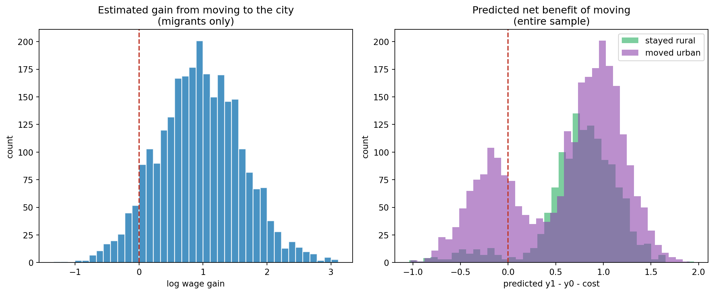
# counterfactual: what would urban workers have earned in the countryside?cf_rural_wage = X @ fiml_beta0 + fiml_rho0 * fiml_sigma0 * mills_1gain = y_obs[migrate ==1] - cf_rural_wage[migrate ==1]fig, axes = plt.subplots(1, 2, figsize=(12, 5))ax = axes[0]ax.hist(gain, bins=40, color='#2980b9', edgecolor='white', alpha=0.85)ax.axvline(0, color='#c0392b', ls='--', lw=1.5)ax.set_title("Estimated gain from moving to the city\n(migrants only)")ax.set_xlabel("log wage gain"); ax.set_ylabel("count")ax = axes[1]# for each person, which sector does the model predict?predicted_gain = (X @ fiml_beta1 - X @ fiml_beta0- (fiml_delta[-2] + fiml_delta[-1] * network))for label, mask, col in [("stayed rural", migrate ==0, '#27ae60'), ("moved urban", migrate ==1, '#8e44ad')]: ax.hist(predicted_gain[mask], bins=40, alpha=0.6, color=col, label=label)ax.axvline(0, color='#c0392b', ls='--', lw=1.5)ax.set_title("Predicted net benefit of moving\n(entire sample)")ax.set_xlabel("predicted y1 - y0 - cost"); ax.set_ylabel("count")ax.legend()plt.tight_layout(); plt.show()print(f"Median estimated gain from moving: {np.median(gain):.3f} log points")print(f"Share of migrants with positive estimated gain: {(gain >0).mean():.1%}")
Median estimated gain from moving: 0.942 log points
Share of migrants with positive estimated gain: 93.0%
The left panel shows the distribution of the estimated treatment effect on the treated: what each migrant gained, relative to what the model says they would have earned had they stayed. If the model is right, most migrants should show a positive gain. The right panel shows the model’s predicted net benefit of moving for everyone (migrants and stayers) and confirms that the model assigns higher predicted gains to those who actually moved.
The role of networks
The exclusion restriction, having a connection in the city, operates through the cost. We can quantify how much it matters:
# predicted migration probability by network status, evaluated at mean Xx_mean = X.mean(axis=0)w_no_net = np.append(x_mean, 0) @ fiml_deltaw_net = np.append(x_mean, 1) @ fiml_deltap_no_net = norm.cdf(w_no_net)p_net = norm.cdf(w_net)print(f"Pr(migrate | no network) = {p_no_net:.1%}")print(f"Pr(migrate | network) = {p_net:.1%}")print(f"Difference: {p_net - p_no_net:.1f} pp")
This is the structural interpretation of the instrument: it does not enter the wage equations, it only shifts the cost, and through the cost it shifts the probability of moving. The exclusion restriction is what lets you separately identify the selection parameters from the wage parameters. Without it, the model is identified only through functional form: the normality assumption alone can in principle separate the regimes, but in practice you want an instrument.
What You Need to Believe
Every structural estimator comes with a list of things you have to accept for the estimates to mean what you claim they mean. Here is the list for the Roy model:
Normality. The joint normality of the errors is doing real work, especially in the FIML estimator. The two-step estimator is more robust: it only needs normality for the probit and a linear conditional expectation for the second stage, but the Mills ratio is still a parametric function. If the wage distribution has fat tails or the selection process is non-normal, the correction can be misleading. A pragmatic check is to compare the two-step and FIML estimates; large discrepancies suggest the normality assumption is strained.
An exclusion restriction. You need at least one variable in \(\mathbf{z}_i\) that affects the migration decision but not the wage. The network variable (a sibling in the city) is the standard one in the migration literature. Other candidates: distance to the nearest urban centre, a push factor like a local harvest failure, or a policy change that lowered moving costs for some groups but not others. Without an exclusion restriction the model is identified only off the nonlinearity of the Mills ratio, and that identification is fragile. The probit is nearly linear over most of its range, so the Mills ratio is nearly collinear with \(\mathbf{x}_i\), and the second-stage estimates become unstable.
No general equilibrium effects. The model treats each person’s potential wages as fixed. If migration is large enough to change urban wages (which in the long run it is) the parameters you estimate are averages over an evolving distribution. This is not a failure of the method so much as a limit on the interpretation of the counterfactuals.
The cost function is correctly specified. You are assuming migration costs are additive and linear in \(\mathbf{z}_i\). If costs also depend on unobservables that are correlated with wage potential. For instance, risk aversion affects both the decision to move and the wage through occupational choice, the error structure is richer than the model allows.
Closing Thoughts
The Roy model is a natural first structural estimator for an economic historian because the question it answers (who selects into what, and what would they have done otherwise) is the question you ask about every major reallocation in history. Who became a factory worker? Who left the land? Who crossed the ocean? The reduced-form difference in means answers none of these convincingly; the Roy model at least tells you the direction and magnitude of the selection, and it forces you to be explicit about what you are assuming to get there.
The two-step estimator is easy to implement, easy to explain, and gives you most of what you need. The FIML estimator sharpens the inference and gives you proper standard errors without bootstrapping. Both are worth having in your toolkit.
The code in this post is a template. Swap in your own \(\mathbf{x}\) and \(\mathbf{z}\), check that the exclusion restriction is defensible, and compare the two-step and FIML estimates as a diagnostic for the normality assumption. The model will not give you a definitive answer (no structural model does), but it will tell you which answer follows from which assumptions, and that is more than the naive comparison can offer.
Footnotes
Roy, A.D. (1951). “Some Thoughts on the Distribution of Earnings.” Oxford Economic Papers, 3(2), 135–146.↩︎
Heckman, J.J. (1979). “Sample Selection Bias as a Specification Error.” Econometrica, 47(1), 153–161.↩︎
Lee, L.-F. (1978). “Unionism and Wage Rates: A Simultaneous Equations Model with Qualitative and Limited Dependent Variables.” International Economic Review, 19(2), 415–433.↩︎
Borjas, G.J. (1987). “Self-Selection and the Earnings of Immigrants.” American Economic Review, 77(4), 531–553.↩︎
Abramitzky, R., Boustan, L.P., and Eriksson, K. (2012). “Europe’s Tired, Poor, Huddled Masses: Self-Selection and Economic Outcomes in the Age of Mass Migration.” American Economic Review, 102(5), 1832–1856.↩︎
A quick way to see this: \(\phi'(t) = -t\,\phi(t)\), since \(\phi(t) = \frac{1}{\sqrt{2\pi}}e^{-t^2/2}\) and the chain rule brings down a \(-t\). So \(\int_c^\infty t\,\phi(t)\,dt = \int_c^\infty -\phi'(t)\,dt = \phi(c)\).↩︎
The likelihood I wrote separates into \(\Pr(I_i) \cdot f(y_i \mid I_i)\). An equivalent and perhaps more familiar form writes the joint density of \((y_{0i}, y_{1i}, I_i^*)\) and integrates out the latent \(I_i^*\), which gives the same expression. See Amemiya, T. (1985). Advanced Econometrics. Harvard University Press, chapter 10.↩︎