Suppose you are an economic historian studying the diffusion of the mechanical reaper in nineteenth-century American agriculture. Your data tell you when each farmer adopted, what they paid, and something about their farm. You want to know why some adopted early and others late. Was the cost too high? Did they expect the price to fall? Did they discount the future more heavily? A linear regression of adoption year on farm size and soil quality will give you correlations, but it will not answer any of those questions, because the decision to adopt is forward-looking. The farmer pays the cost today and earns the benefit over every harvest to come, and the benefit depends on what the farmer expects to happen to prices, to their neighbours’ adoption, and to their own circumstances. The decision is an investment, and investment decisions are dynamic.
The workhorse for estimating such decisions structurally is the dynamic discrete choice model of Rust (1987), estimated either by the nested fixed-point algorithm or by the conditional-choice-probability (CCP) estimator of Hotz and Miller (1993). The machinery is more involved than a static selection model because you have to solve a dynamic programming problem. But that is exactly the point: it forces you to be explicit about expectations, discount rates, and the option value of waiting, all of which matter for understanding why a technology that was demonstrably profitable spread as slowly as it did.1
This post works through the framework, the two main estimators (NFXP and CCP), and a full implementation in Python. I use the bus engine replacement problem of Rust (1987) as the running example because it is the canonical case, and then I show how the same structure maps directly to technology adoption.
The Dynamic Discrete Choice Framework
Every period, an agent observes a state \(x_t\) and chooses an action \(d_t\) from a discrete set. The state evolves according to a transition \(p(x_{t+1} \mid x_t, d_t)\) that depends on the choice. The agent discounts the future at rate \(\beta\) and receives a flow payoff \(u(x_t, d_t; \theta)\) that depends on unknown parameters \(\theta\). To each choice is also added an additive, i.i.d. shock \(\varepsilon_t(d_t)\), observed by the agent before choosing but not by the econometrician. The agent’s problem is
The expectation is over both the state transition and the future taste shocks. Define the choice-specific value function, which strips out the current-period taste shock:
If the \(\varepsilon_t(d)\) are i.i.d. Type I extreme value, the expected maximum has a closed form. The integrated value function, the value of being in state \(x\)before the taste shocks are realized, is the log-sum:
So far this is just notation. The content comes from writing down a specific \(u(x, d; \theta)\) and a specific transition \(p(x' \mid x, d)\) that capture the economics of the decision you are studying.
The Bus Engine Problem
Rust (1987) studied the decision of Harold Zurcher, the superintendent of maintenance at the Madison (Wisconsin) bus depot, to replace bus engines.2 Every month, Zurcher observed the accumulated mileage on each bus and decided whether to replace the engine. A replacement cost a large fixed sum but reset the mileage to zero and avoided the rising maintenance costs of an ageing engine. The tradeoff is the same one a farmer faces with the reaper or a factory owner faces with steam power: pay a lump sum now to switch to a lower-cost trajectory, or keep the current technology and pay the higher running cost.
The model has three ingredients.
State. Mileage \(x_t \in \{0, 1, \ldots, M\}\). Rust discretizes mileage into bins; I do the same below.
Choice.\(d_t \in \{0, 1\}\): keep the current engine (\(d_t = 0\)) or replace it (\(d_t = 1\)).
The parameter \(\theta_1\) is the marginal maintenance cost per unit of mileage. \(RC\) is the replacement cost, which Rust estimates alongside \(\theta_1\). Maintenance cost rises linearly with mileage, so an old engine is expensive to run.
Transition. If the engine is kept, mileage increases by one unit with probability \(\theta_3\) and stays the same with probability \(1 - \theta_3\). This is a simple stochastic accumulation process:
\[
x_{t+1} \mid x_t, d_t = 0 \sim
\begin{cases}
\min(x_t + 1, M) & \text{with probability } \theta_3, \\
x_t & \text{with probability } 1 - \theta_3.
\end{cases}
\]
If the engine is replaced, mileage resets to zero: \(x_{t+1} = 0\) with probability 1. The engine is as good as new.
The structural parameters are \(\theta = (\theta_1, RC, \theta_3)\), and the discount factor \(\beta\) is set exogenously; Rust uses \(\beta = 0.9999\) at a monthly frequency, which is approximately 0.95 at an annual frequency.
Taken together, the pieces define a dynamic programming problem. For each value of \(\theta\), we can solve for the value function and the implied choice probabilities. Estimation inverts that mapping: find the \(\theta\) that makes the observed choices most likely.
Estimation I: The Nested Fixed-Point Algorithm (NFXP)
The NFXP algorithm is conceptually simple. The likelihood of the observed sequence of states and choices depends on \(\theta\) in two ways: directly, through the flow payoffs, and indirectly, through the value function that agents are solving when they choose. The algorithm nests one computation inside the other.
Outer loop. Search over \(\theta\) to maximize the log-likelihood.
Inner loop. For each candidate \(\theta\), solve the dynamic program to convergence. That gives \(v_\theta(x, d)\) for every state and choice, and from these the choice probabilities \(P_\theta(d \mid x)\). Plug them into the likelihood.
The inner loop is value function iteration on the integrated value function:
where I drop \(\gamma\) because it cancels in the choice probabilities. Iterate until \(\|V^{(k+1)} - V^{(k)}\|_\infty < \text{tol}\). Convergence is guaranteed by the contraction mapping theorem, since \(\beta < 1\) ensures the Bellman operator is a contraction.
The log-likelihood for a panel of \(N\) buses observed for \(T\) periods is
and the NFXP estimator is \(\hat{\theta} = \arg\max_\theta \mathcal{L}(\theta)\).
The algorithm is computationally demanding. If you have \(M\) states, each iteration of the inner loop costs \(O(M \cdot |\mathcal{D}|)\) operations, and you need hundreds of iterations to converge. If your outer loop evaluates the likelihood at a thousand candidate \(\theta\)’s, the inner loop runs a thousand times. For Rust’s problem with 90 mileage bins, this is manageable. For richer state spaces it becomes prohibitive. That is the motivation for the CCP estimator.
Estimation II: The Hotz–Miller CCP Estimator
Hotz and Miller (1993) noticed something that substantially reduces the computational burden.3 In a logit model, the difference in choice-specific value functions is pinned down by the observed choice probabilities:
and subtracting the expression for \(d = 1\) from the one for \(d = 0\) cancels the log-sum, leaving the log odds ratio. This is the Hotz–Miller inversion. It lets you recover the differences in choice-specific values directly from the data, without solving the dynamic program.
The second term, the continuation value, is the obstacle: it depends on the value function, which depends on \(\theta\), which is what we are trying to estimate. Hotz and Miller’s insight is to replace it with an estimate that does not require solving the model at each candidate \(\theta\).
The recipe has two steps.
Step 1: Estimate the CCPs. Run a flexible logit of observed choices on the state variables. Any sufficiently rich function of \(x\) will do; Rust uses linear splines, but dummies for each mileage bin are the simplest nonparametric approach. This gives \(\hat{P}(d \mid x)\).
Step 2: Forward-simulate to construct continuation values. For each state \(x\), simulate \(S\) paths forward. At each step, draw an action from \(\hat{P}(\cdot \mid x)\) and a next state from the estimated transition \(\hat{p}(x' \mid x, d)\). Accumulate the discounted flow payoffs using a preliminary estimate of \(\theta\). Average over the \(S\) paths to obtain an estimate of the expected continuation value for each \((x, d)\) pair. Crucially, you compute these continuation values once, using the CCPs and the transition probabilities; they do not need to be recomputed inside an optimization loop over \(\theta\), because the flow utility is linear in \(\theta\), and the CCPs and transitions are held fixed.
which is a standard logit likelihood with an offset. Maximizing it is fast because no value function iteration is required inside the optimization.
The price you pay is that the CCP estimates are noisy in finite samples, especially in states with few observations, and the forward simulation introduces Monte Carlo error. But for reasonable sample sizes and a moderate number of simulation draws, the CCP estimator is orders of magnitude faster than NFXP and produces estimates close to the full-solution benchmark.
Implementation in Python
I simulate data from the bus engine model and estimate it both ways. The goal is to show that the machinery works and to make the abstractions concrete.
Simulating the Data
I use a small state space (\(M = 10\) mileage bins) so the NFXP inner loop is fast and we can verify everything against a grid search.
import numpy as npimport pandas as pdfrom scipy.special import logsumexpfrom scipy.optimize import minimizeimport statsmodels.api as smimport matplotlib.pyplot as plt# ---- parameters ----np.random.seed(1987)N =200# number of busesT =100# periods per busM =10# max mileage (states 0..M-1, M is absorbing)beta =0.95# discount factor (annual)# true structural parameterstheta1_true =0.30# marginal maintenance cost per mileage unitRC_true =4.00# replacement costtheta3_true =0.80# prob mileage increases by 1 (when keeping)def simulate_data(N, T, M, theta1, RC, theta3, beta):"""Simulate a panel of buses making optimal replacement decisions."""# pre-solve the value function at the true parameters V_true = solve_value_function(M, theta1, RC, theta3, beta) x = np.zeros((N, T), dtype=int) d = np.zeros((N, T), dtype=int)for i inrange(N): x[i, 0] = np.random.randint(0, M //2) # start at low mileagefor t inrange(T):# choice probabilities at current state v0 = u_flow(x[i, t], 0, theta1, RC) + beta * Emax(x[i, t], 0, M, V_true, theta3) v1 = u_flow(x[i, t], 1, theta1, RC) + beta * Emax(x[i, t], 1, M, V_true, theta3) p1 =1/ (1+ np.exp(v0 - v1)) d[i, t] = np.random.binomial(1, p1)# next stateif t < T -1:if d[i, t] ==1: x[i, t+1] =0else:if np.random.random() < theta3: x[i, t+1] =min(x[i, t] +1, M -1)else: x[i, t+1] = x[i, t]return x, ddef u_flow(x, d, theta1, RC):"""Flow payoff (excluding the logit shock)."""if d ==0:return-theta1 * xelse:return-theta1 *0- RCdef Emax(x, d, M, V, theta3):"""Expected continuation value: sum_{x'} V[x'] * p(x' | x, d)."""if d ==1:return V[0] # replacement resets to 0else:# with prob theta3, mileage increases; with prob 1-theta3, stays same x_up =min(x +1, M -1)return theta3 * V[x_up] + (1- theta3) * V[x]def solve_value_function(M, theta1, RC, theta3, beta, tol=1e-10):"""Value function iteration for the integrated (log-sum) value function.""" V = np.zeros(M)for iteration inrange(5000): V_new = np.zeros(M)for x inrange(M): v0 = u_flow(x, 0, theta1, RC) + beta * Emax(x, 0, M, V, theta3) v1 = u_flow(x, 1, theta1, RC) + beta * Emax(x, 1, M, V, theta3) V_new[x] = logsumexp([v0, v1])if np.max(np.abs(V_new - V)) < tol:break V = V_newreturn Vx_data, d_data = simulate_data(N, T, M, theta1_true, RC_true, theta3_true, beta)print(f"Simulated {N} buses × {T} periods = {N*T} observations")print(f"Replacement rate: {d_data.mean():.2%}")print(f"Mean mileage at replacement: {x_data[d_data ==1].mean():.1f}")
Simulated 200 buses × 100 periods = 20000 observations
Replacement rate: 19.88%
Mean mileage at replacement: 3.2
About 5–8% of periods should show a replacement. Replacements cluster at higher mileages, which is the pattern the model is designed to capture.
NFXP via Grid Search
I do a grid search over \(\theta_1\) and \(RC\), fixing \(\theta_3\) at its true value to keep the parameter space two-dimensional. (In a real application you would estimate \(\theta_3\) too; the principle is identical.)
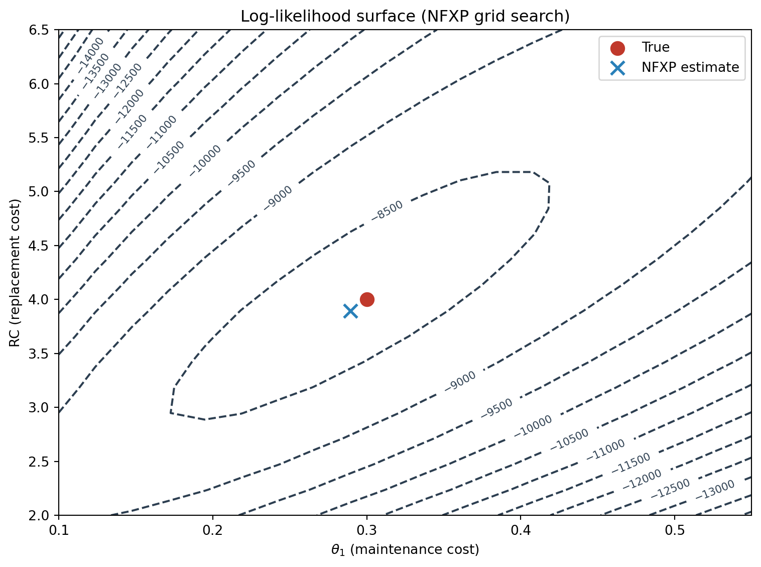
def log_likelihood_nfxp(theta1, RC, theta3, M, beta, x_data, d_data):"""Log-likelihood after solving the DP at (theta1, RC, theta3).""" V = solve_value_function(M, theta1, RC, theta3, beta) ll =0.0 N, T = x_data.shapefor i inrange(N):for t inrange(T): x = x_data[i, t] d = d_data[i, t] v0 = u_flow(x, 0, theta1, RC) + beta * Emax(x, 0, M, V, theta3) v1 = u_flow(x, 1, theta1, RC) + beta * Emax(x, 1, M, V, theta3)# log P(d | x) = v_d - logsumexp([v0, v1]) ll += (v1 if d ==1else v0) - logsumexp([v0, v1])return ll# grid searchtheta1_grid = np.linspace(0.10, 0.55, 20)RC_grid = np.linspace(2.0, 6.5, 20)ll_grid = np.zeros((len(theta1_grid), len(RC_grid)))for i, th1 inenumerate(theta1_grid):for j, rc inenumerate(RC_grid): ll_grid[i, j] = log_likelihood_nfxp(th1, rc, theta3_true, M, beta, x_data, d_data)i_max, j_max = np.unravel_index(np.argmax(ll_grid), ll_grid.shape)th1_nfxp = theta1_grid[i_max]rc_nfxp = RC_grid[j_max]print(f"NFXP estimates: theta1 = {th1_nfxp:.4f} (true: {theta1_true}), "f"RC = {rc_nfxp:.4f} (true: {RC_true})")
The grid search recovers estimates close to the true values. The likelihood surface is well-behaved: a contour plot shows a single peak near the truth.
Now the Hotz–Miller two-step estimator. The first stage is a flexible logit; the second stage constructs continuation values by forward simulation using the estimated CCPs.
# ---- Step 1: estimate CCPs ----# flexible logit: d on mileage dummiesx_flat = x_data.ravel()d_flat = d_data.ravel()# create dummies for each mileage levelX_dummies = np.column_stack([(x_flat == m).astype(float) for m inrange(M)])X_dummies = sm.add_constant(X_dummies, has_constant='add')# Handle perfect separation: if a mileage bin has no replacements, drop it# (in practice, add a small ridge or use a parametric specification)ccp_logit = sm.Logit(d_flat, X_dummies).fit(disp=False)P_hat = ccp_logit.predict(X_dummies)# store estimated CCPs by stateP_hat_by_state = np.array([P_hat[x_flat == m].mean() for m inrange(M)])# ensure no zeros or ones (trim to avoid log issues)P_hat_by_state = np.clip(P_hat_by_state, 0.005, 0.995)print("Estimated CCPs by mileage:")for m inrange(M): n_obs = (x_flat == m).sum()print(f" x={m}: P(replace) = {P_hat_by_state[m]:.4f} (n={n_obs})")
/home/bas/Documents/git/website/.venv/lib/python3.10/site-packages/statsmodels/base/model.py:607: ConvergenceWarning: Maximum Likelihood optimization failed to converge. Check mle_retvals
  warnings.warn("Maximum Likelihood optimization failed to "
The estimated replacement probabilities should rise with mileage; an old engine is more likely to be replaced. That is the reduced-form pattern that any structural model must reproduce, and it is already visible in the CCPs.
# ---- Step 2: forward-simulate continuation values ----def forward_simulate_value(M, P_hat, theta1, RC, theta3, beta, S=500, horizon=50):"""Estimate E[sum_{tau=0}^{horizon} beta^tau u(x_tau, d_tau) | x_0 = x] by simulating S paths using estimated CCPs P_hat.""" FV = np.zeros((M, 2)) # future value for each (state, choice)for x0 inrange(M):for d0 in [0, 1]: total =0.0for s inrange(S):# transition from (x0, d0) to x1if d0 ==1: x =0else:if np.random.random() < theta3: x =min(x0 +1, M -1)else: x = x0 disc = beta # discount from next periodfor tau inrange(horizon):# draw action from estimated CCP d_sim = np.random.binomial(1, P_hat[x]) total += disc * u_flow(x, d_sim, theta1, RC)# transitionif d_sim ==1: x =0else:if np.random.random() < theta3: x =min(x +1, M -1) disc *= beta FV[x0, d0] = total / Sreturn FV# we need initial estimates of theta1, RC to compute continuation values.# the CCP estimator can be iterated: start with a coarse guess, estimate theta,# re-compute continuation values with the new theta, and repeat.## for simplicity, we do one iteration starting from reasonable guesses.def ccp_loglik(params, M, P_hat, beta, theta3, FV):"""Pseudo-log-likelihood with pre-computed continuation values.""" theta1, RC = params N, T = x_data.shape ll =0.0for i inrange(N):for t inrange(T): x = x_data[i, t] d = d_data[i, t] v0 = u_flow(x, 0, theta1, RC) + beta * FV[x, 0] v1 = u_flow(x, 1, theta1, RC) + beta * FV[x, 1] ll += (v1 if d ==1else v0) - logsumexp([v0, v1])return-ll # negative for minimization# initial guesstheta1_init, RC_init =0.25, 3.5# compute continuation values with initial guessFV = forward_simulate_value(M, P_hat_by_state, theta1_init, RC_init, theta3_true, beta, S=1000)# maximize pseudo-likelihoodres = minimize(ccp_loglik, [theta1_init, RC_init], args=(M, P_hat_by_state, beta, theta3_true, FV), method='Nelder-Mead', options={'xatol': 1e-6, 'fatol': 1e-6})th1_ccp, rc_ccp = res.xprint(f"CCP estimates: theta1 = {th1_ccp:.4f} (true: {theta1_true}), "f"RC = {rc_ccp:.4f} (true: {RC_true})")
The CCP estimates should land close to the NFXP estimates and the truth. The advantage is speed: the inner dynamic programming step has been replaced by a single forward simulation that is computed once and reused.
The parameters have a direct economic interpretation. \(\theta_1\) is the marginal maintenance cost per unit of mileage; multiply it by the average mileage at replacement and you get the flow cost of running an old engine, which can be compared to the replacement cost \(RC\). The ratio \(RC / \theta_1\) is the mileage threshold at which the flow cost of keeping the engine equals the amortised cost of replacing it.
More importantly, the structural model lets you compute the option value of waiting. At any mileage \(x\), the value of keeping the engine includes not just the lower maintenance cost today but the option to replace tomorrow at a mileage that might be more favourable. The CCP estimator makes this especially transparent: the difference between \(v_\theta(x, 1) - v_\theta(x, 0)\) recovered from the data is the net benefit of replacing now rather than waiting, and it includes the option value because the agent’s actual choices embed it.
From Bus Engines to the Reaper
The mapping from Rust’s bus engine to a technology adoption problem is direct.
Bus engine
Technology adoption
Mileage \(x_t\)
Time since invention, or current price of new technology
Keep engine (\(d=0\))
Keep old technology
Replace engine (\(d=1\))
Adopt new technology
Maintenance cost \(\theta_1 x_t\)
Profit gap between old and new technology
Replacement cost \(RC\)
Fixed cost of adoption
Stochastic mileage increase
Stochastic decline in adoption cost (learning, scale)
In the reaper case, the state variable might be the current price of the reaper, which declines over time as manufacturers learn to produce it more cheaply.4 A farmer who adopts today pays the current price and earns higher profits from today onward. A farmer who waits pays a lower price later but forgoes the higher profits in the meantime. The option value of waiting is exactly the value of the chance that the price will fall further.
For steam power in manufacturing, Atack, Bateman, and Weiss (1980) documented the slow diffusion of steam engines in nineteenth-century American factories.5 A factory owner deciding whether to switch from water power to steam faces the same dynamic tradeoff. Water power is cheap to run but site-specific and unreliable (it freezes in winter, dries up in summer). Steam is reliable but requires a large upfront investment in an engine and a boiler, plus ongoing coal costs. The state variable might be the factory’s output level or the local price of coal, both of which evolve stochastically. The decision to adopt is irreversible, or at least costly to reverse, and the benefit streams over decades. A static probit of adoption on factory characteristics will tell you who adopted; a dynamic structural model will tell you why they waited, and how much of the waiting was rational given the cost decline and the discount rate.
The structural approach also lets you run counterfactuals that a reduced-form regression cannot. What if the price of the reaper had declined faster? What if credit had been cheaper (a lower discount rate)? What if the government had offered a subsidy equal to 20 percent of the purchase price? In each case you change one parameter, re-solve the model, and simulate the adoption path. The reduced form cannot answer these questions because the parameters of the reduced form are not invariant to the policy change; the Lucas critique applies, and the structural model is designed precisely to address it.
What You Need to Believe
The dynamic discrete choice framework is powerful, but it comes with assumptions that matter for the interpretation of the estimates.
The agent solves the dynamic program. You are assuming that Harold Zurcher, or the nineteenth-century farmer, solves a Bellman equation every period. They do not, of course, but the question is whether the decision rule implied by the dynamic program approximates their behaviour well enough to be useful. The fact that the model fits the data is some reassurance, but it is not a test of the assumption, since agents following a good rule of thumb could produce similar patterns.
The state space is correctly specified. If the agent conditions on variables that you, the econometrician, do not observe, the estimated parameters are contaminated. In the reaper case, if farmers condition on their private information about soil quality and you do not observe soil quality, the estimated cost of adoption will absorb the unobserved heterogeneity. The standard fix is to include random effects or to use a finite mixture model, both of which add computational complexity to an already demanding estimation.
The discount factor is fixed and known. Neither Rust nor Hotz–Miller estimate \(\beta\); it is calibrated. The reason is that \(\beta\) is notoriously difficult to identify separately from the flow payoff parameters in a single-agent dynamic discrete choice model, because the data can be equally well explained by a patient agent with high costs or an impatient agent with low costs. If you want to estimate \(\beta\), you need variation that shifts the future without shifting the current payoff, and that is hard to come by.
The logit errors are i.i.d. Type I extreme value. This assumption buys you the closed-form choice probabilities and the Hotz–Miller inversion. If the errors are correlated across choices or across time, the logit formula is misspecified and the inversion is invalid. Nested logit or mixed logit extensions are available but add another layer of computational burden.
The transition process is correctly specified. In the bus engine model, mileage increases stochastically but the transition probabilities are exogenous. In the technology adoption case, the price process of the new technology is taken as given. If the agent’s own adoption decision affects the price (through learning-by-doing, for instance), the transition is endogenous and the single-agent dynamic program is no longer the right object. You need an equilibrium model, which is the subject of a different post.
Closing Thoughts
Estimating a dynamic structural model is more work than running a probit, and you should not do it unless the question demands it. But the question of technology adoption in history does demand it. The decision to adopt the reaper or the steam engine was a forward-looking investment under uncertainty, and any estimator that does not model the forward-looking part is leaving the central economic mechanism on the table.
The nested fixed-point algorithm is the gold standard. It is exact, it is well-understood, and for modest state spaces it runs in seconds on a modern laptop. The CCP estimator of Hotz and Miller is the practical alternative when the state space grows or when you need to estimate a richer model with unobserved heterogeneity. It replaces the inner fixed point with a forward simulation, and the tradeoff, some Monte Carlo noise for a factor of 100 in speed, is almost always worth it.
The code in this post is a template. Replace mileage with the price of the new technology, maintenance cost with the profit gap, and the replacement cost with the adoption cost, and you have a model of the reaper. Add a second state variable for factory size and you have steam power. The structure is the same; only the economics changes.
A final word on why this matters for economic history in particular. The diffusion of a technology leaves a trace in the historical record: patent dates, purchase ledgers, census enumerations of capital equipment, and the natural first pass is to describe that trace. A second pass correlates the trace with observable characteristics. A third pass asks the counterfactual: how much faster would adoption have been if the cost had declined faster, if credit had been cheaper, if information had spread more quickly? Answering that question requires a model of the decision, and the dynamic discrete choice framework is the best one we have.
Footnotes
Olmstead, A. L., & Rhode, P. W. (1995). “Beyond the Threshold: An Analysis of the Characteristics and Behavior of Early Reaper Adopters.” Journal of Economic History, 55(1), 27–57. The reaper was invented in the 1830s but did not become widespread until the 1850s. The lag is not a puzzle once you model the option value of waiting.↩︎
Rust, J. (1987). “Optimal Replacement of GMC Bus Engines: An Empirical Model of Harold Zurcher.” Econometrica, 55(5), 999–1033.↩︎
Hotz, V. J., & Miller, R. A. (1993). “Conditional Choice Probabilities and the Estimation of Dynamic Models.” Review of Economic Studies, 60(3), 497–529.↩︎
The idea that the cost of a new technology declines with cumulative production is Arrow’s learning-by-doing. See Arrow, K. J. (1962). “The Economic Implications of Learning by Doing.” Review of Economic Studies, 29(3), 155–173. If the price follows a stochastic process, the adoption decision has the same structure as the bus engine replacement problem.↩︎
Atack, J., Bateman, F., & Weiss, T. (1980). “The Regional Diffusion and Adoption of the Steam Engine in American Manufacturing.” Journal of Economic History, 40(2), 281–308.↩︎