Unified Growth Theory: How an Economy Escapes the Malthusian Trap

Author

Bas Machielsen

Published

June 15, 2026

Introduction

For most of recorded history, income per capita barely changed. It fluctuated around a roughly constant subsistence level, and the gains from any technological improvement were absorbed, within a few generations, by a larger population. Then, over the last two centuries, some economies broke out of this pattern and moved onto sustained growth, while others did so later or not at all. Plotted over time, world GDP per capita is roughly flat for millennia and then rises steeply.

A unified theory of growth tries to account for this entire trajectory with a single model: the long Malthusian stagnation, the escape from it, the demographic transition, and the divergence in incomes across countries. This is the aim of Unified Growth Theory (UGT), developed mainly by Oded Galor and co-authors.¹

The feature of the model I want to focus on is that the escape is not driven by an external shock or an exogenous regime change. It comes from the same forces that sustain the Malthusian regime. The slow accumulation of population gradually changes the structure of the dynamical system until the Malthusian equilibrium ceases to exist. In the language of dynamical systems, a slowly moving state variable drives the system through a saddle-node bifurcation.

The plan is to set out each step of the argument — formally and intuitively — and then implement the dynamical system in Python and simulate the take-off.

The Malthusian world

Before we can appreciate the escape, we need to understand the trap. The Malthusian logic rests on three ingredients:

A subsistence constraint. People need a minimum consumption \(\tilde c\) to survive. Anything above subsistence can be spent on having and raising children.
A positive effect of income on population. When income rises above subsistence, families can afford more surviving children, so the population grows: \(y \uparrow \;\Rightarrow\; L \uparrow\).
A fixed factor — land. Output is produced with labor and a fixed quantity of land. More workers on the same land means diminishing average product: \(L \uparrow \;\Rightarrow\; AP_L \downarrow \;\Rightarrow\; y \downarrow\).

Put these together and you get a powerful negative feedback loop. Suppose a new technology raises productivity. In the very short run, income rises above subsistence. In the short run, higher income means more children, so the population grows. But in the long run, a larger population spread over fixed land drives the average product of labor — and hence income — back down to subsistence. The fruits of progress are converted into people, not into living standards.

The key consequence: technological progress in a Malthusian world shows up as population density, not as income per capita. A more productive region (better land, better technology) is not richer per person; it is merely more crowded. Income per capita is pinned, in the long run, to a subsistence-determined constant.

Production

Let us write this down. There is an overlapping-generations economy, \(t = 0, 1, 2, \dots\), producing one homogeneous good with two factors: labor measured in efficiency units, \(H_t\), and a fixed quantity of land, \(X\). Output is

\[ Y_t = H_t^{\alpha}\,(A_t X)^{1-\alpha}, \qquad \alpha \in (0,1), \]

where \(A_t\) is the level of technology. Dividing by the number of workers \(L_t\) gives output per worker:

\[ y_t = h_t^{\alpha}\, x_t^{1-\alpha}, \]

where

\[ h_t \equiv \frac{H_t}{L_t} \quad (\text{efficiency units per worker}), \qquad x_t \equiv \frac{A_t X}{L_t} \quad (\text{effective resources per worker}). \]

The variable \(x_t\) is central to the model. It is effective land per person: the stock of land, scaled up by technology \(A_t\), divided across the population \(L_t\). Because land \(X\) is fixed, \(x_t\) rises when technology improves (\(A_t \uparrow\)) and falls when the population grows (\(L_t \uparrow\)). The Malthusian trade-off between progress and crowding operates through this ratio.

The three mechanisms of change

A purely Malthusian model stagnates indefinitely. UGT adds three mechanisms that accumulate in the background and eventually overturn the Malthusian regime. I’ll state each as a qualitative relationship (a function with sign restrictions), because it is the comparative statics — not the exact functional form — that drive the results.

Engine 1: Technology responds to scale and to education

The rate of technological progress between \(t\) and \(t+1\),

\[ g_{t+1} \equiv \frac{A_{t+1} - A_t}{A_t} = g(e_t, L_t), \]

depends on two things: the education \(e_t\) of the current generation and the size \(L_t\) of the population. The assumptions are

\[ g_e > 0,\quad g_{ee} < 0, \qquad g_L > 0,\quad g_{LL} < 0, \qquad g(0, L) > 0 \text{ for } L > 0. \]

The intuition:

Population size matters (\(g_L > 0\)). In early stages of development, more people means more potential innovators, more demand for new goods, more diffusion of ideas, finer division of labor, and more trade. A larger society generates faster technological progress — the scale effect. This is the channel through which the accumulation of population eventually matters.
Education matters (\(g_e > 0\)). In later stages, educated individuals are better at creating and adopting new technologies. This is the channel through which human capital feeds back into progress.
Progress is positive even with no education (\(g(0,L) > 0\)). Technology advances through trial and error and learning-by-doing even in an illiterate society, so the scale effect is always operating.
Both effects are diminishing (\(g_{ee}, g_{LL} < 0\)).

Engine 2: Human capital responds to technological change

An individual joining the workforce in period \(t+1\) has human capital

\[ h_{t+1} = h(e_{t+1}, g_{t+1}), \]

with the following sign restrictions:

\[ h_e > 0,\; h_{ee} < 0; \qquad h_g < 0,\; h_{gg} > 0; \qquad h_{eg} > 0; \qquad h(0,g) > 0. \]

The crucial and somewhat subtle assumptions are the ones involving \(g\):

Technological change erodes human capital (\(h_g < 0\)). In a rapidly changing technological environment, existing skills become obsolete. The weaver’s expertise is worthless once the power loom arrives.
Education shields against obsolescence (\(h_{eg} > 0\)). This is the heart of the matter. Education is most valuable precisely when technology is changing fast, because an educated person can adapt — re-learn, re-tool, reallocate. When \(g\) is low (a static world), education has little payoff; when \(g\) is high (a dynamic world), education becomes essential.

This complementarity between education and technological change is what converts an acceleration in \(g\) into a demand for human capital. It is the hinge on which the whole transition turns.

Engine 3: Households choose quantity and quality of children

This is where the demographic transition comes from. Individuals live for two periods. As children they consume a fraction of their parents’ time. As adults they supply labor, have children, decide how much to educate each child, and consume.

Raising a child takes time: a fixed amount \(\tau\) regardless of quality, plus \(e_{t+1}\) extra units of time to give the child education \(e_{t+1}\). So a child of quality \(e_{t+1}\) costs \(\tau + e_{t+1}\) units of parental time. An adult \(t\) has preferences

\[ u^t = (1-\gamma)\ln(c_t) + \gamma \ln\!\big(n_t\, h_{t+1}\big), \]

where \(c_t\) is own consumption, \(n_t\) is the number of children, and \(h_{t+1}\) is the human capital (the quality) of each child. Note that parents care about the product \(n_t h_{t+1}\) — they value both how many children they have and how capable each one is. This single term is what makes the quantity–quality trade-off possible.

The budget constraint says that the time (equivalently, potential income \(z_t\)) spent on children plus own consumption cannot exceed potential income:

\[ z_t\, n_t (\tau + e_{t+1}) + c_t \le z_t, \qquad z_t \equiv y_t = h_t^{\alpha} x_t^{1-\alpha}, \]

and there is the subsistence floor

\[ c_t \ge \tilde c. \]

Solving the household’s problem

Let me now derive the optimal choices completely, because the structure of the solution is the economics. Define the fraction of (potential) income devoted to children,

\[ \rho_t \equiv n_t (\tau + e_{t+1}), \]

so that \(c_t = z_t (1 - \rho_t)\). Substituting \(n_t = \rho_t / (\tau + e_{t+1})\) and \(c_t = z_t(1-\rho_t)\) into the utility function, and using \(\ln(n_t h_{t+1}) = \ln \rho_t - \ln(\tau + e_{t+1}) + \ln h(e_{t+1},g_{t+1})\), the objective becomes

\[ u^t = (1-\gamma)\ln\!\big(z_t(1-\rho_t)\big) \;+\; \gamma \ln \rho_t \;+\; \gamma\,\Big[\ln h(e_{t+1}, g_{t+1}) - \ln(\tau + e_{t+1})\Big]. \]

Look closely: the choice variables separate. The first two terms involve only \(\rho_t\) (how much total to spend on children), and the last bracket involves only \(e_{t+1}\) (the quality of each child). We can optimize them one at a time.

Step 1 — Optimal child quality (education)

Maximizing the last bracket means maximizing \(\dfrac{h(e_{t+1}, g_{t+1})}{\tau + e_{t+1}}\) over \(e_{t+1} \ge 0\). The first-order condition is

\[ \frac{h_e(e_{t+1}, g_{t+1})}{h(e_{t+1}, g_{t+1})} = \frac{1}{\tau + e_{t+1}}. \]

The left side is the proportional return to an extra unit of education; the right side is its proportional cost in parental time. Set them equal and you get the optimal education, which depends only on the rate of technological progress:

\[ e_{t+1} = e(g_{t+1}) = \begin{cases} 0 & \text{if } g_{t+1} \le \hat g, \\[4pt] > 0,\ e'(g_{t+1}) > 0 & \text{if } g_{t+1} > \hat g. \end{cases} \]

This threshold property is the qualitative engine of the take-off, and it follows directly from the human-capital assumptions. When technology is nearly static (\(g_{t+1} \le \hat g\)), obsolescence is not a concern, the marginal return to education \(h_e\) is too low to justify its time cost, and parents choose the corner solution \(e_{t+1} = 0\) — no education at all. Only once technological progress exceeds the threshold \(\hat g\) does education start to pay, and from then on parents invest more in education the faster technology changes (\(e'(g) > 0\), because \(h_{eg} > 0\)).

Step 2 — Optimal child quantity (the subsistence regimes)

Now maximize over \(\rho_t\), the total resources devoted to children, subject to \(c_t = z_t(1-\rho_t) \ge \tilde c\). Ignoring the constraint for a moment, the first-order condition of \((1-\gamma)\ln(z_t(1-\rho_t)) + \gamma \ln \rho_t\) is

\[ -\frac{1-\gamma}{1-\rho_t} + \frac{\gamma}{\rho_t} = 0 \quad\Longrightarrow\quad \rho_t = \gamma. \]

So in the unconstrained case the household spends a constant fraction \(\gamma\) of its resources on children and consumes \(c_t = (1-\gamma)z_t\). This is valid only if consumption clears subsistence, \((1-\gamma)z_t \ge \tilde c\), i.e. only if potential income exceeds the threshold

\[ \tilde z \equiv \frac{\tilde c}{1-\gamma}. \]

If instead \(z_t < \tilde z\), the subsistence constraint binds: the household consumes exactly \(c_t = \tilde c\) and devotes everything left over to children, \(\rho_t = 1 - \tilde c / z_t\). Collecting both cases:

\[ \rho_t = n_t(\tau + e_{t+1}) = \begin{cases} \gamma & \text{if } z_t \ge \tilde z \quad (\text{unconstrained}), \\[4pt] 1 - \dfrac{\tilde c}{z_t} & \text{if } z_t \le \tilde z \quad (\text{subsistence binds}). \end{cases} \]

Dividing through by the cost-per-child \(\tau + e(g_{t+1})\) gives the fertility rule:

\[ n_t = \begin{cases} \dfrac{\gamma}{\tau + e(g_{t+1})} \equiv n^{b}(g_{t+1}) & \text{if } z_t \ge \tilde z, \\[10pt] \dfrac{1 - \tilde c / z_t}{\tau + e(g_{t+1})} \equiv n^{a}(g_{t+1}, z_t) & \text{if } z_t \le \tilde z. \end{cases} \]

Two features of this solution are worth noting:

In the Malthusian region (\(z_t \le \tilde z\), and \(g_{t+1} \le \hat g\) so \(e = 0\)), fertility is \(n_t = (1 - \tilde c / z_t)/\tau\), which is increasing in income \(z_t\). Richer Malthusian families have more children. This is the positive income–population link behind the trap.
In the modern region (\(z_t \ge \tilde z\)), fertility is \(n_t = \gamma / (\tau + e(g_{t+1}))\), which is decreasing in education. Once technology changes fast enough to make \(e > 0\), every additional unit of child quality raises the cost of a child and so reduces the optimal number of children. This is the quantity–quality trade-off, and it produces the demographic transition: rising demand for human capital pulls fertility down.

Assembling the dynamical system

We can now write the laws of motion. Population evolves through fertility,

\[ L_{t+1} = n_t L_t, \]

and effective resources per worker evolve through the race between technology and population,

\[ x_{t+1} = \frac{A_{t+1} X}{L_{t+1}} = \frac{(1 + g_{t+1}) A_t X}{n_t L_t} = \frac{1 + g_{t+1}}{n_t}\, x_t. \]

This last equation is worth pausing on. Resources per worker grow when technology outruns population, \(1 + g_{t+1} > n_t\), and shrink otherwise. In the Malthusian steady state these exactly balance: fertility adjusts until \(n_t = 1 + g_{t+1}\), so \(x_t\) — and therefore income — is constant. The escape from stagnation is, mechanically, the moment when \(g\) accelerates and \(n\) collapses, so that \((1+g)/n\) jumps well above one and \(x\) begins to compound.

Putting all four state variables together, the economy is a sequence \(\{x_t, e_t, g_t, L_t\}_{t=0}^{\infty}\) satisfying

\[ \boxed{ \begin{aligned} x_{t+1} &= \phi(e_t, g_t, x_t, L_t)\, x_t, \\ e_{t+1} &= e\big(g(e_t, L_t)\big), \\ g_{t+1} &= g(e_t, L_t), \\ L_{t+1} &= n(e_t, g_t, x_t, L_t)\, L_t. \end{aligned}} \]

This is a four-dimensional nonlinear dynamical system. Its essential behavior can be understood by isolating a two-dimensional subsystem, which is where the take-off mechanism lives.

The conditional dynamics of technology and education

Notice the structure of the middle two equations:

\[ g_{t+1} = g(e_t, L_t), \qquad e_{t+1} = e(g_{t+1}). \]

The pair \((g, e)\) evolves on its own, driven only by the population size \(L\): education and growth interact without any input from income or resources. So we can hold \(L\) fixed at some level and study the conditional subsystem. Substituting one equation into the other, education obeys a one-dimensional map:

\[ e_{t+1} = E(e_t; L) \equiv e\big(g(e_t, L)\big). \]

Its steady states are the fixed points \(e^* = E(e^*; L)\). The geometry is as follows:

\(g(e, L)\) is increasing and concave in \(e\), and it shifts up as \(L\) rises (because \(g_L > 0\)). More people \(\Rightarrow\) faster progress at every level of education.
\(e(g)\) is flat at zero until \(g\) exceeds the threshold \(\hat g\), then rises and eventually saturates. Education only switches on in a sufficiently dynamic environment.

Compose these two and the map \(E(\cdot; L)\) is S-shaped: flat near the origin, then steep, then saturating. An S-shaped map crossing the \(45^\circ\) line can intersect it one, two, or three times, and which of these happens depends on the height of the \(g\)-curve — that is, on \(L\).

This gives three qualitatively different regimes:

Small population. The \(g\)-curve is low; even fully educated, society cannot push \(g\) much above \(\hat g\). The only fixed point is the Malthusian one at \(e^* = 0\): no education, slow technology, stagnation. It is locally stable, and it is the only attractor. The economy is trapped.
Intermediate population. The \(g\)-curve has risen enough that the high branch appears. Now there are three fixed points: a stable Malthusian state \(e^L \approx 0\), an unstable threshold \(e^u\), and a stable modern-growth state \(e^H\) with high education and fast progress. The unstable point \(e^u\) is the dividing line: start below it and the economy returns to stagnation; start above it and it converges to sustained growth. A small economy sitting at \(e^L = 0\) stays trapped, but the basin of that trap, the interval \([0, e^u)\), shrinks as \(L\) grows.
Large population. The \(g\)-curve is now high enough that \(g(0, L) > \hat g\): even with zero education, technology changes fast enough to make education worthwhile. The Malthusian fixed point at \(e = 0\) no longer exists — it has collided with the unstable point \(e^u\) and both have disappeared. Only the modern-growth steady state \(e^H\) remains, and every economy converges to it regardless of where it starts.

This is the phase transition. As \(L\) increases, the stable Malthusian equilibrium and the unstable threshold move toward each other, merge, and disappear — a saddle-node (fold) bifurcation. This is the point made in the introduction, now stated precisely:

In the Malthusian regime income stays near subsistence, but population is not constant. It rises slowly, generation after generation, because the scale effect keeps technological progress above zero. This accumulation of \(L\) is what pushes the conditional \(g\)-curve upward, until the Malthusian equilibrium the economy occupies ceases to exist. The escape is not triggered from outside the model; it follows from the Malthusian dynamics themselves.

Once the Malthusian state is gone, education becomes positive, the demand for human capital rises, fertility falls through the quantity–quality channel, population growth declines, \((1+g)/n\) rises above one, and income per capita starts to grow.

The next sections work through this in code.

Building the dynamical system in Python

We need explicit functional forms that respect the qualitative assumptions above. I’ll use the following, which satisfy every sign restriction:

\[ g(e, L) = g_{\max}\,\frac{\eta_L L^{\rho} + \eta_e e}{1 + \eta_L L^{\rho} + \eta_e e}, \qquad \rho \in (0,1), \]

a bounded, increasing, concave function of both arguments with \(g(0,L) > 0\);

\[ e(g) = e_{\max}\,\frac{\max(g - \hat g, 0)^{p}}{\kappa^{p} + \max(g - \hat g, 0)^{p}}, \qquad p > 1, \]

a smooth S-shaped response that is exactly zero below the threshold \(\hat g\) and rises convexly then saturates above it; and a human-capital function in which technology erodes skills but education shields against the erosion (\(h_{eg} > 0\)),

\[ h(e, g) = \max\!\left(\underline h,\; 1 + \theta_e e - \frac{\theta_g\, g}{1 + \theta_{eg} e}\right). \]

import numpy as np
import matplotlib.pyplot as plt

# ---- structural parameters ----
params = dict(
    alpha = 0.45,   # human-capital share in output
    gamma = 0.70,   # weight on children in utility
    tau   = 0.298,  # time cost per child (quantity)
    ctil  = 1.00,   # subsistence consumption
    # technology  g(e, L)
    g_max = 0.60, rho = 0.50, eta_L = 0.0016, eta_e = 3.0,
    # education   e(g)
    ghat = 0.05, e_max = 0.45, kappa = 0.10, p = 2.0,
    # human capital h(e, g)
    th_e = 1.5, th_g = 2.0, th_eg = 4.0, h_min = 0.05,
)
params["ztil"] = params["ctil"] / (1 - params["gamma"])   # income s.t. subsistence just binds

def g_tech(e, L, pr=params):
    """Rate of technological progress g(e, L): increasing & concave in e and L, g(0,L)>0."""
    X = pr["eta_L"] * L**pr["rho"] + pr["eta_e"] * e
    return pr["g_max"] * X / (1 + X)

def e_edu(g, pr=params):
    """Optimal education e(g): zero below the threshold ghat, S-shaped above it."""
    d = np.maximum(g - pr["ghat"], 0.0)
    return pr["e_max"] * d**pr["p"] / (pr["kappa"]**pr["p"] + d**pr["p"])

def h_cap(e, g, pr=params):
    """Human capital h(e, g): rises with education, eroded by g, education shields (h_eg>0)."""
    return np.maximum(pr["h_min"], 1 + pr["th_e"]*e - pr["th_g"]*g / (1 + pr["th_eg"]*e))

Visualizing the phase transition

First let’s draw the conditional map \(E(e; L) = e\big(g(e, L)\big)\) against the \(45^\circ\) line for three population sizes, and mark the steady states. This is the picture that contains the whole story.

def cond_map(e, L):
    return e_edu(g_tech(e, L))

def fixed_points(L, pr=params):
    """All steady states of e -> E(e;L) on [0, e_max], classified as stable/unstable."""
    grid = np.linspace(0, pr["e_max"] * 1.02, 200001)
    f = cond_map(grid, L) - grid
    sign = np.sign(f)
    cross = np.where(sign[:-1] * sign[1:] < 0)[0]
    pts = []
    # e = 0 is a steady state whenever g(0,L) <= ghat  (so E(0)=0)
    if g_tech(0.0, L) <= pr["ghat"]:
        pts.append((0.0, "stable"))
    for i in cross:
        r = grid[i]
        h = 1e-4
        slope = (cond_map(r + h, L) - cond_map(max(r - h, 0), L)) / (2 * h)
        pts.append((r, "stable" if abs(slope) < 1 else "unstable"))
    return pts

L_values = [500, 3000, 8000]
titles = ["Small population (trapped)",
          "Intermediate population (3 equilibria)",
          "Large population (Malthusian state gone)"]

e_grid = np.linspace(0, params["e_max"] * 1.02, 400)
fig, axes = plt.subplots(1, 3, figsize=(15, 4.6))
for ax, L, title in zip(axes, L_values, titles):
    ax.plot(e_grid, cond_map(e_grid, L), color="#c0392b", lw=2,
            label=r"$E(e;L)=e(g(e,L))$")
    ax.plot(e_grid, e_grid, "k--", lw=1, alpha=0.6, label=r"$45^\circ$ line")
    for e_star, kind in fixed_points(L):
        ax.plot(e_star, e_star, "o", ms=10,
                mfc=("white" if kind == "unstable" else "#2c3e50"),
                mec="#2c3e50", mew=1.6, zorder=5)
    ax.set_title(f"{title}\n$L = {L}$", fontsize=10)
    ax.set_xlabel(r"$e_t$"); ax.set_ylabel(r"$e_{t+1}$")
    ax.legend(loc="upper left", fontsize=8); ax.grid(alpha=0.3)
plt.tight_layout(); plt.show()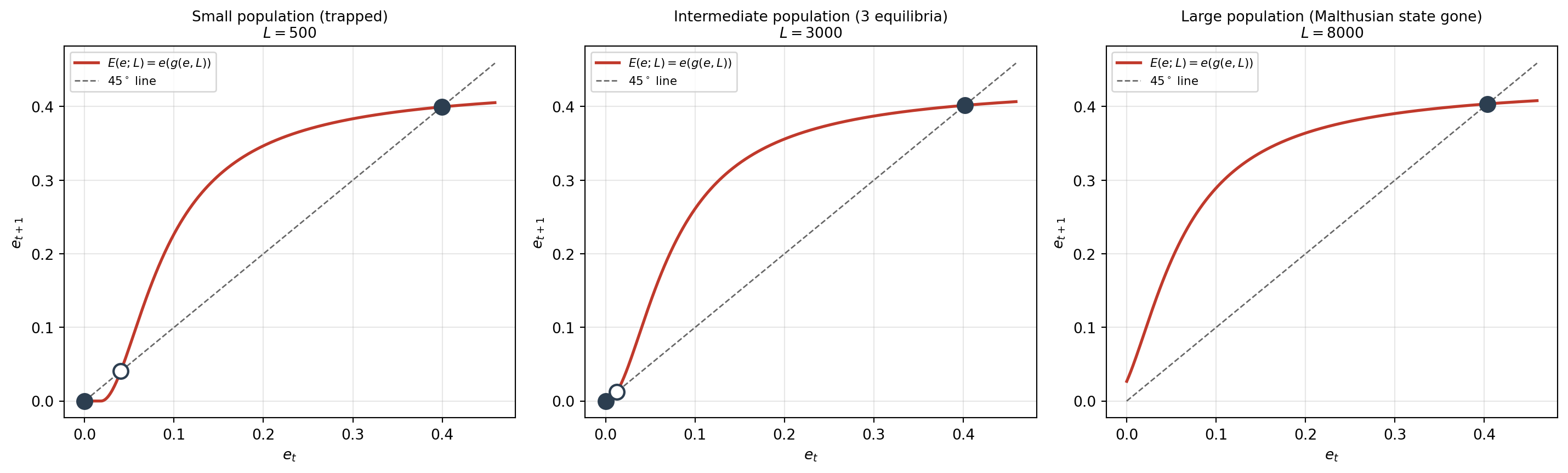

Filled dots are stable steady states; the open dot is the unstable threshold \(e^u\). Reading left to right: a small economy has only the trapped state at \(e = 0\); an intermediate economy has the trap, the threshold, and a modern-growth state; and a large economy has only the modern-growth state, the Malthusian equilibrium having disappeared.

Iterating the map: convergence to the trap vs. take-off

To see the dynamics, we can iterate the map directly. Starting from some \(e_0\), we step between the map and the \(45^\circ\) line to trace the trajectory \(e_0, e_1, e_2, \dots\). At the intermediate \(L\), whether the economy ends up trapped or takes off depends on which side of the unstable threshold \(e^u\) it starts.

def iterate_path(ax, L, e0, color):
    e = e0
    for _ in range(60):
        e_next = cond_map(e, L)
        ax.plot([e, e], [e, e_next], color=color, lw=1)            # vertical: read off the map
        ax.plot([e, e_next], [e_next, e_next], color=color, lw=1)  # horizontal: back to 45 line
        if abs(e_next - e) < 1e-9:
            break
        e = e_next

L = 3000
fig, ax = plt.subplots(figsize=(7, 6))
ax.plot(e_grid, cond_map(e_grid, L), color="#c0392b", lw=2, label=r"$E(e;L)$")
ax.plot(e_grid, e_grid, "k--", lw=1, alpha=0.6, label=r"$45^\circ$ line")
iterate_path(ax, L, e0=0.010, color="#2980b9")   # just below threshold -> returns to the trap
iterate_path(ax, L, e0=0.030, color="#27ae60")   # just above threshold -> takes off
for e_star, kind in fixed_points(L):
    ax.plot(e_star, e_star, "o", ms=11,
            mfc=("white" if kind == "unstable" else "#2c3e50"),
            mec="#2c3e50", mew=1.6, zorder=5)
ax.set_title(f"Iterating $e_{{t+1}}=E(e_t;L)$ at $L = {L}$")
ax.set_xlabel(r"$e_t$"); ax.set_ylabel(r"$e_{t+1}$")
ax.legend(loc="upper left"); ax.grid(alpha=0.3)
plt.tight_layout(); plt.show()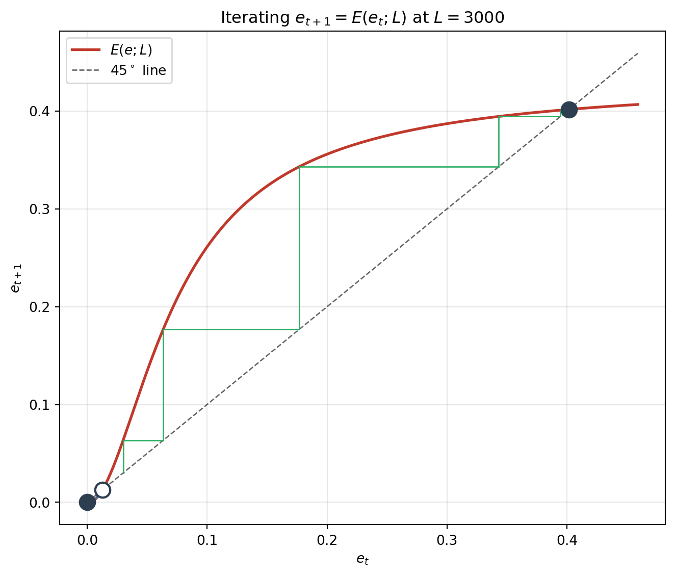

The blue path starts just below the threshold and converges down to the Malthusian state at \(e = 0\). The green path starts just above it and converges to the modern-growth equilibrium. The two are separated by the unstable fixed point \(e^u\). As \(L\) rises, \(e^u\) moves toward zero, the blue basin shrinks, and at the critical population it disappears: there is no longer any region below the threshold from which the economy can fall back.

The bifurcation diagram

We can summarize the entire phase transition in one plot: the steady-state education level as a function of population \(L\). This is the bifurcation diagram of the conditional system.

L_scan = np.linspace(200, 9000, 700)
stable_pts, unstable_pts = [], []
for L in L_scan:
    for e_star, kind in fixed_points(L):
        (stable_pts if kind == "stable" else unstable_pts).append((L, e_star))

stable_pts = np.array(stable_pts)
unstable_pts = np.array(unstable_pts)

fig, ax = plt.subplots(figsize=(9, 5.2))
ax.scatter(stable_pts[:, 0], stable_pts[:, 1], s=4, color="#2c3e50",
           label="stable steady state")
ax.scatter(unstable_pts[:, 0], unstable_pts[:, 1], s=4, color="#c0392b",
           label="unstable threshold $e^u$")
ax.set_title("Bifurcation diagram: the Malthusian equilibrium vanishes as $L$ grows")
ax.set_xlabel("population size $L$ (frozen)")
ax.set_ylabel(r"steady-state education $e^*$")
ax.legend(); ax.grid(alpha=0.3)
plt.tight_layout(); plt.show()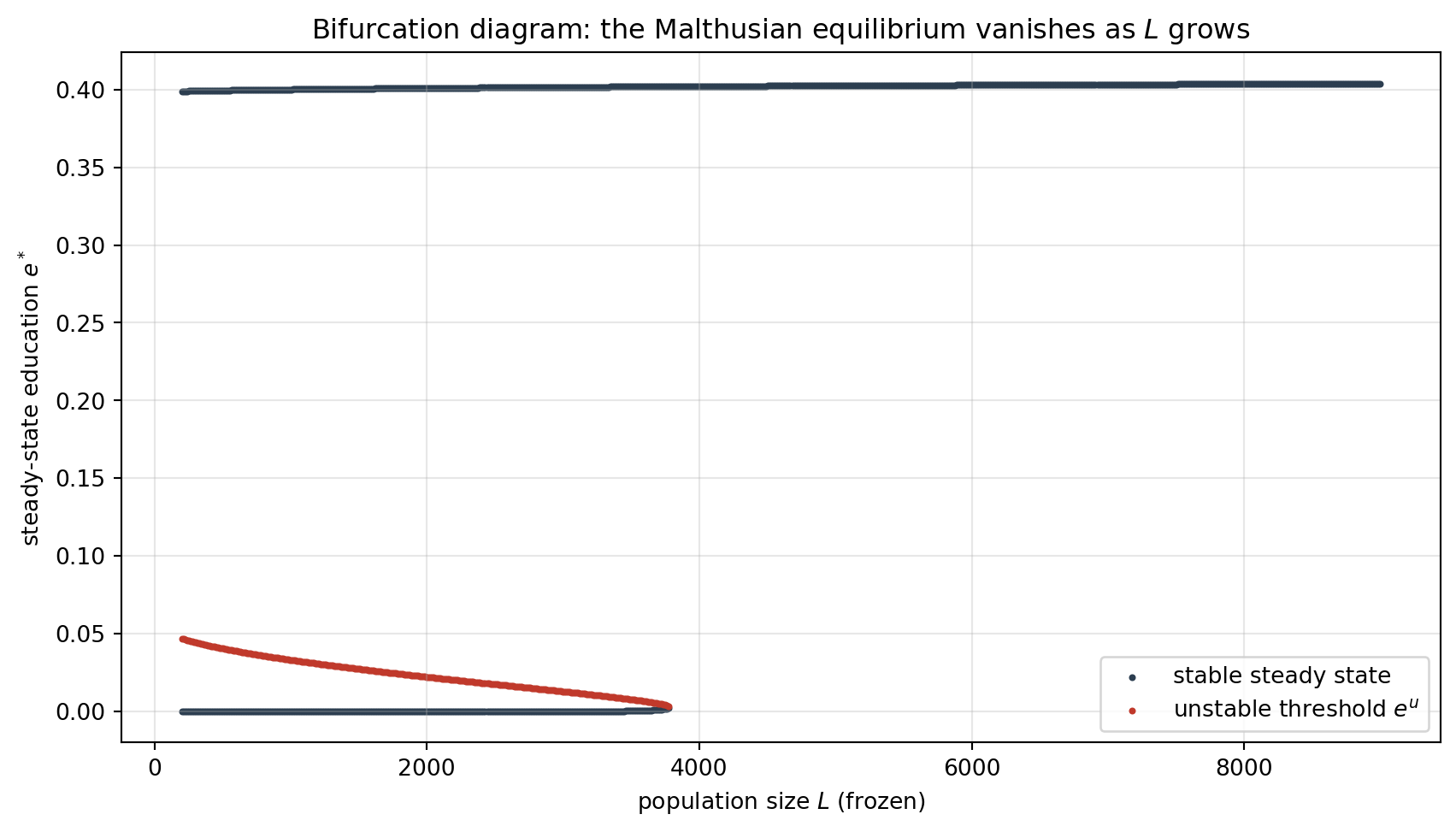

The lower stable branch (the Malthusian state, \(e^* = 0\)) and the unstable branch curving up from it meet and terminate at a critical population size. To the right of that point only the upper branch — the modern-growth equilibrium — remains. An economy on the lower branch, as \(L\) slowly increases, reaches the bifurcation, at which point the Malthusian equilibrium no longer exists and the economy converges to the modern-growth state.

The full simulation

The conditional analysis tells us what happens to \((g, e)\) for each \(L\). To see it play out in historical time we let all four state variables move together: population \(L\) accumulates slowly in the Malthusian era and moves the conditional system toward its bifurcation, and once the take-off begins, income \(x\) and education \(e\) rise sharply while fertility \(n\) falls.

def simulate(T=320, L0=150.0, x0=1.85, pr=params):
    L = np.zeros(T); e = np.zeros(T); g = np.zeros(T); x = np.zeros(T)
    y = np.zeros(T); n = np.zeros(T); h = np.zeros(T)
    L[0], x[0], e[0] = L0, x0, 0.0
    g[0] = g_tech(0.0, L0)
    for t in range(T - 1):
        h[t] = h_cap(e[t], g[t])
        y[t] = h[t]**pr["alpha"] * x[t]**(1 - pr["alpha"])   # potential income z_t = y_t
        z = y[t]
        g_next = g_tech(e[t], L[t])          # technology depends on CURRENT education & population
        e_next = float(e_edu(g_next))        # education responds to next period's progress
        # fraction of resources spent on children: subsistence regime vs. unconstrained regime
        rho = pr["gamma"] if z >= pr["ztil"] else 1 - pr["ctil"] / z
        n[t] = rho / (pr["tau"] + e_next)
        L[t+1] = n[t] * L[t]
        x[t+1] = (1 + g_next) / n[t] * x[t]
        e[t+1], g[t+1] = e_next, g_next
    h[-1] = h_cap(e[-1], g[-1])
    y[-1] = h[-1]**pr["alpha"] * x[-1]**(1 - pr["alpha"])
    n[-1] = n[-2]
    return dict(L=L, e=e, g=g, x=x, y=y, n=n)

sim = simulate()
takeoff = int(np.argmax(sim["e"] > 0.05))
print(f"Take-off occurs at generation t = {takeoff}, "
      f"when population reaches L = {sim['L'][takeoff]:.0f}")

Take-off occurs at generation t = 159, when population reaches L = 4696

t = np.arange(len(sim["y"]))
fig, axes = plt.subplots(2, 2, figsize=(13, 9))

# Income per capita -- the hockey stick (log scale)
ax = axes[0, 0]
ax.semilogy(t, sim["y"], color="#c0392b", lw=2)
ax.axvline(takeoff, color="gray", ls=":", lw=1)
ax.set_title("Income per capita $y_t$ (log scale): the hockey stick")
ax.set_xlabel("generation $t$"); ax.set_ylabel(r"$y_t$"); ax.grid(alpha=0.3)

# Population
ax = axes[0, 1]
ax.plot(t, sim["L"], color="#2980b9", lw=2)
ax.axvline(takeoff, color="gray", ls=":", lw=1)
ax.set_title("Population $L_t$: slow Malthusian rise, then plateau")
ax.set_xlabel("generation $t$"); ax.set_ylabel(r"$L_t$"); ax.grid(alpha=0.3)

# Education and technological progress
ax = axes[1, 0]
ax.plot(t, sim["e"], color="#27ae60", lw=2, label=r"education $e_t$")
ax.plot(t, sim["g"], color="#8e44ad", lw=2, label=r"tech. progress $g_t$")
ax.axvline(takeoff, color="gray", ls=":", lw=1)
ax.set_title("Education and technological progress switch on together")
ax.set_xlabel("generation $t$"); ax.legend(); ax.grid(alpha=0.3)

# Fertility -- the demographic transition
ax = axes[1, 1]
ax.plot(t, sim["n"], color="#d35400", lw=2)
ax.axhline(1.0, color="gray", ls="--", lw=1, alpha=0.7)
ax.axvline(takeoff, color="gray", ls=":", lw=1)
ax.set_title("Fertility $n_t$: the demographic transition")
ax.set_xlabel("generation $t$"); ax.set_ylabel(r"$n_t$"); ax.grid(alpha=0.3)

plt.tight_layout(); plt.show()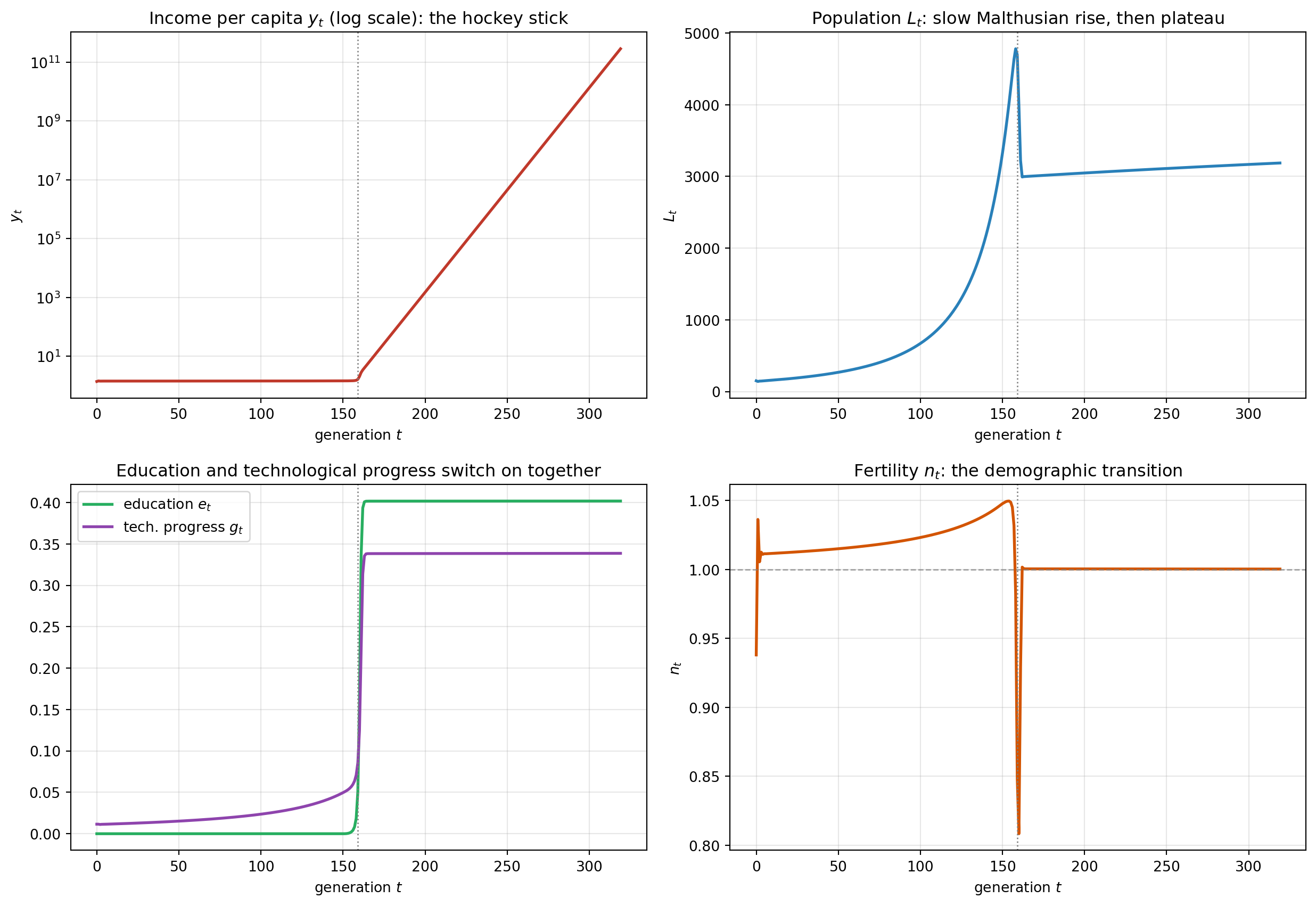

The four panels together trace the model’s account of long-run growth:

The Malthusian epoch (left of the dotted line, roughly 150 generations). Education is zero, technological progress is slow, and income per capita is flat — it stays near a subsistence-determined constant with a negligible trend. Population is nonetheless rising throughout, because the scale effect keeps \(g\) slightly positive and fertility slightly above replacement. Little appears to change in income, but \(L\) is accumulating.
The take-off. Once \(L\) crosses the critical level, the conditional Malthusian equilibrium disappears, education rises off zero, and the education–technology feedback takes over: more education raises \(g\), faster \(g\) raises the return to education, which raises \(e\) further. Within a few generations the economy moves from \(e \approx 0\) to its modern level.
The demographic transition. As education becomes valuable, the quantity–quality trade-off operates: each child now carries an education cost, so fertility falls. Population growth slows to replacement and \(L\) levels off.
Sustained growth. With population growth at replacement, \((1 + g)/n\) settles above one, so effective resources per worker \(x_t\) — and hence income \(y_t\) — grow without bound. Progress is no longer offset by population growth and instead passes through into income per capita. On the log scale, income becomes an approximately straight, upward-sloping line.

Note that no parameter changes during the simulation: the same model that produces the long stagnation also ends it. The escape is a property of the Malthusian dynamics, not of an external change.

Comparative development: why some economies took off first

The same model accounts for cross-country divergence. The timing of the take-off depends on how high the conditional \(g\)-curve sits and on how readily education responds, and these depend on country-specific characteristics. Galor writes technology and education as

\[ g_{t+1}^{i} = g\big(e_t^{i}, L_t^{i}, \Omega_t^{i}\big), \qquad e_{t+1}^{i} = e\big(g_{t+1}^{i}; \Psi_t^{i}\big), \]

where \(\Omega^{i}\) collects features that make a country good at generating technological progress — protection of property rights, the stock of knowledge, openness to trade and the technological diffusion it brings, innovation-friendly culture and institutions, population diversity, and the local availability of complementary resources (coal for the steam engine, say). A higher \(\Omega\) shifts the \(g\)-curve up, so the saddle-node bifurcation arrives at a smaller population — the country escapes the trap earlier.

The term \(\Psi^{i}\) collects features that govern human-capital formation — the ability to finance education and forgone earnings, the availability and quality of public schooling, cultural and religious attitudes toward literacy, the disease environment that determines the return to investing in a child’s future, and the social status of education. A more education-friendly \(\Psi\) lowers the threshold \(\hat g(\Psi)\) at which education switches on, so the human-capital response — and hence the demographic transition and the growth take-off — comes sooner.

Two countries, \(A\) and \(B\), identical except that \(B\) has slightly more favorable \(\Omega\) or \(\Psi\), reach the bifurcation at different dates. A small difference in the timing of the take-off compounds into a large gap in income, because once an economy is on the modern-growth branch its income grows exponentially. In this account, variation in the timing of the take-off is the proximate source of the divergence in incomes over the last two centuries, and deep-rooted geographic, cultural, and institutional factors are what set that timing.

Concluding remarks

Unified Growth Theory uses a single dynamical system, with no regime switches imposed by hand, to reproduce

the long Malthusian epoch, in which income per capita stagnates while technology and population rise together;
an endogenous escape, driven by the accumulation of population, that removes the Malthusian equilibrium through a saddle-node bifurcation rather than through an external shock;
the rise of human capital and the demographic transition, both following from the quantity–quality trade-off once technology accelerates; and
the divergence across countries, governed by the timing of the take-off and hence by deep-rooted characteristics.

The central point is that the same Malthusian forces that hold income down — in particular the scale effect of population on technological progress — also raise the conditional growth curve over time until the Malthusian equilibrium no longer exists. The model is worth setting out in full, and simulating, because the escape from stagnation is a consequence of the stagnation itself rather than an assumption added on top.

Footnotes

The canonical references are Galor and Weil (2000, AER) and Galor (2011), Unified Growth Theory, Princeton University Press. This post follows the structure of a lecture by Ömer Özak on Economic Growth and Comparative Development, and reconstructs the dynamical system at its core.↩︎