Project Organization and Structured Data with LLMs
Andromeda Workshop
Introduction
Introduction
- Bas Machielsen (a.h.machielsen@uu.nl)
- Assistant Professor in Applied Economics at UU
- Teach various classes:
- Introduction to Applied Data Science (BSc 1st year)
- Applied Economics Research Course (BSc 3rd year)
- Empirical Economics (MSc)
- Research: Economic history & Political economy
- Lots of unstructured data (historical documents)
- And lots of econometric challenges
- Use machine learning and AI on a daily basis to solve these problems
Outline
- Preliminaries
- Motivation
- Setting up
- Positron
- Python
- R
- Organizating a project
- Structuring Data with LLMs
- Econometric analysis
- Conclusion
Preliminaries
- I want to talk about a boring subject: project organization.
- However, because project organization is so boring, I will try to illustrate the use of this with a spontaneous project.
- The project will answer an economic research question through the use of publicly available data, which I web scrape and structure through LLMs.
- If you have an OpenAI developer account (or something else you can use) and some spare balance (you don’t need more than 1/2 euros for this)1, feel free to tag along and run the code alongside me.
- If you don’t, I have uploaded the data provided to us by the LLM, so you can still tag along.
- Download links are in the remainder of the presentation.
Motivation
- Why project organization?
- Reproducibility: This addresses the question: Can another person take your exact code and data and arrive at the same results? It focuses on the computational consistency of your work.
- Replication: This asks: If another analyst independently tries to answer the same question, will they reach a similar conclusion? This speaks to the robustness and generalizability of the findings themselves.
- Transparency: This ensures that all the choices you made and the methods you employed are clearly documented and accessible to others. It’s about showing your work to build trust and allow for scrutiny.
- Efficiency: Familiarizing yourself with a workflow helps you to work and collaborate more efficiently with others.
- Efficiency is the big elephant in the room here. I think many people work very inefficiently using very inefficient tools. I want to change that.
In Academia
- In academia: the academic community increasingly emphasizes the importance of reproducibility to uphold the integrity of scientific findings.
- Establishing Trust: Many research findings have failed to be replicated, leading to a “replication crisis” that undermines confidence in scientific outcomes.
- Enabling Collaboration and Advancement: When research is reproducible, others can confidently build upon your work, enhancing collaboration and accelerating scientific progress.
- Meeting Modern Publishing Standards: A growing number of journals now mandate that a complete “replication package,” including all data and code, be submitted alongside a manuscript.
- Promoting Transparency through Open Science: The push for greater transparency and reproducibility is a cornerstone of the open science movement. This movement advocates for making scientific research, data, and dissemination accessible to everyone.
In Business
- In the corporate world, collaborative and sustainable practices are paramount. Reproducible work is essential for:
- Collaboration: Your code and analyses must integrate flawlessly with the work of your colleagues.
- Scalability: Sometimes your code and work has to be used by tens, hundreds or (tens of) thousands of individuals.
- Long-Term Maintainability: Eventually, others will inherit your projects. Reproducibility ensures a smooth transition and allows them to build upon your contributions effectively.
Set Up
Prerequisites
- Download and install Positron (here)
- Positron is a new IDE (the successor of RStudio) that “(..) unifies exploration and production work in one free, AI-assisted environment, empowering the full spectrum of data science in Python and R.”
- In other words, it’s going to be good at both Python and R
- I think both of these languages are the future of data science
- Ability to smoothly work with both useful in whatever you’re going to do.
- For people familiar with VSCode and/or RStudio, Positron is basically a combination of the two.
Python
- Before installing Python (don’t worry if you already have Python), I’d like you to install the
uvpackage manager.- This is a competitor of
conda, which is often used. - However
condais very mediocre IMO and you often run into dependency issues.
- This is a competitor of
uvis available here.- You have to open a terminal and copy+paste the command to install
uv
- You have to open a terminal and copy+paste the command to install
uvis very good at managing Python packages and their versions such that all packages are compatible with each other- The logic is that for each separate project, you’ll set-up a Python “environment” that is isolated from the rest of your system: specific versions of several packages that are compatible with each other.
- In addition,
uvis just faster and more straightforward compared toconda.
Set-up uv
- For each new project you ever do with Python, you create a new folder somewhere on your system.
- After downloading & installing
uv, you set-up a Python environment inside this folder. This is accomplished using three subsequent commands in the terminal:
- After
uv unit,uvwill create the following files with information about your project:
├── .gitignore
├── .python-version
├── README.md
├── main.py
└── pyproject.toml
Set-up uv
- After
uv venv,uvwill create a virtual environment allowing it to run Python code independently from all other python versions on your system.1- Some fundamental Python libraries already come pre-integrated with the virtual environment. However, other than those, the environment is completely empty, so you’d have to install basic packages manually (more later).
- The final thing you do is activating the virtual environment:
source .venv/bin/activatein the terminal.- Alternatively, in Positron or VSCode, press
CTRL+P, typeInterpreter: Discover All Interpretersand select your virtual environment on the top right of your screen. See here also.
- Alternatively, in Positron or VSCode, press
- For a more extensive guide, see here.
Installing Python Libraries
- Now we can proceed adding Python to our newly-created environment. For this workshop, we only need a couple of them. This is super simple:
uv add numpy polars chatlas dotenvThis command will do two things:
- Install the package to this virtual environment (so not to all other Python distributions you might have on your system)
- Write some information to some of the project-related files we created with
uv initto ensure that the documentation contains the instructions about which packages and which versions have just been installed.
numpyandpolarsare standard data wrangling libraries,chatlasis a library that allows us to interact easily with LLMs.
R Set-Up
- R is a little bit easier to set-up, but it is more difficult to isolate virtual environments in R.
- It is possible to do so using the
venvR packages, but in this presentation, we will just use our global R environment.
- It is possible to do so using the
- For R, we’ll need the
tidyverse,ellmerpackages.tidyversedoes the data wrangling,ellmerdoes the interaction with LLMs.
Positron Introduction
Organizing a Project
Positron and Projects
From the Positron Website:
Expert data scientists keep all the files associated with a given project together — input data, scripts, analytical results, and figures. This is such a wise and common practice, in data science and in software development more broadly, that most integrated development environments (IDEs) have built-in support for this practice.
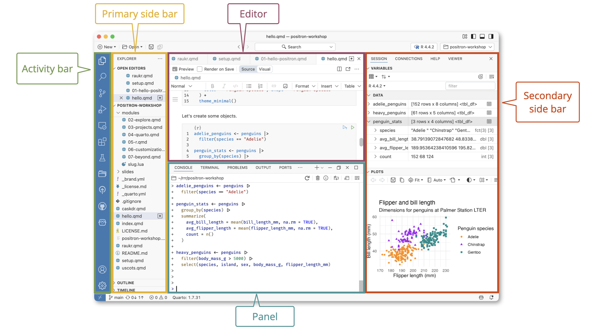
- The concept in Positron that’s most analogous to an RStudio Project is a workspace and this is inherited directly (and intentionally) from VS Code.
- A Positron (or VS Code) workspace is often just a project folder that’s been opened in its own window via Open Folder or similar.
Six Subtopics
File Organization Principle I
Every data science project you do should be in one folder. Everything you use in this project (reports, data, the programming environment, output, etc.) should be inside that folder.. or on the web. But not elsewhere on your system.
- What should that folder and its contents look like?
- Code organization
- File organization
- Version control
- Abstraction
- Commenting
- Unit tests
Literature and General Principles
Ristovska (2019): Coding for Economists: A Language-Agnostic Guide
Gentzkow and Shapiro (2014): Code and Data for the Social Sciences: A Practitioner’s Guide
McDermott (2020): Data Science for Economists
Hagerty (2020): Advanced Data Analytics in Economics
General principles:
- Make things easier for your future self or collaborators.
- Don’t trust your future self.
File Organization
File Organization Principle II
Use separate directories by function. Separate files into inputs and outputs. Always use relative filepaths (“../input/data.csv” instead of “C:/build/input/data.csv”). Define your working directory interactively.
- Why?
- Easily find what you’re looking for.
- Protect your raw data from being saved over.
- Most importantly, others can run your code on their own computer with minimal changes.
File Organization [2]
- Folder structure (
my_projectis the folder you open in Positron):
/my_project
  /rawdata
  /code
    /1_clean
    /2_process
    /3_results
  /preppeddata
  /output
    /tables
    /figures
/temp- In the main folder (root directory), place:
- A README file that gives a basic overview of your project. E.g. detail variable names and sources.
- A master script that lists and runs all other scripts.
Code Organization
Code Organization Principle
Break programs into short scripts or functions, each of which conducts a single task.
Make names distinctive and meaningful.
Be consistent with code style and formatting.
- Directory structure
- Code and comment style
- File naming conventions
- Variable naming conventions
- Use the same output data structure
Why?
- Your own working memory is limited.
- You will forget everything in 1-2 weeks.
- Writing out what your script will do helps you think better.
- Your collaborators need to be able to easily understand your code.
Example Code Organization
- Note that in Python we describe the function using a docstring, and in R, we use Roxygen2 documentation.
def calculate_average_word_length(text_input: str) -> float:
    """Calculates the average length of words in a given text.

    This function takes a string of text, splits it into individual words,
    and then computes the average length of those words. Punctuation is
    handled by a separate helper function.

    Args:
        text_input: A string containing the text to be analyzed.

    Returns:
        A floatExample Code Organization representing the average word length. Returns 0.0 if the
        input string is empty or contains no words.
    """
    # Helper function to remove punctuation from a single word.
    def _clean_word(word: str) -> str:
        punctuation_to_remove = ".,!?;:"
        return ''.join(char for char in word if char not in punctuation_to_remove)

    # Return 0.0 immediately if the input is not a string or is empty.
    if not isinstance(text_input, str) or not text_input:
        return 0.0

    cleaned_words = [_clean_word(word) for word in text_input.split()]

    # Filter out any empty strings that might result from cleaning.
    non_empty_words = [word for word in cleaned_words if word]

    if not non_empty_words:
        return 0.0

    total_length = sum(len(word) for word in non_empty_words)
    word_count = len(non_empty_words)

    return total_length / word_count

# Example of how to run this.

# 1. Define a sample sentence.
sentence = "Programs are meant to be read by humans, and only incidentally for computers to execute."

# 2. Call the function with the sample sentence.
average_length = calculate_average_word_length(sentence)

# 3. Print the result to see the output.
print(f"The average word length is: {average_length:.2f}")
## The average word length is: 4.80
#' Calculate the Average Length of Words in a Given Text
#'
#' @description
#' This function takes a character string, removes common punctuation, splits the
#' string into individual words, and then computes the average length of those words.
#'
#' @param text_input A character string containing the text to be analyzed.
#'
#' @return A numeric value representing the average word length. Returns 0
#' if the input is invalid, empty, or contains no words after cleaning.
#'
#' @examples
#' sentence <- "Programs are meant to be read by humans, and only incidentally for computers to execute."
#' calculate_avg_word_length(sentence)
#'
calculate_avg_word_length <- function(text_input) {
# 1. Input Validation
# Immediately return 0 if the input is not a single, non-empty string.
if (!is.character(text_input) || length(text_input) != 1 || nchar(text_input) == 0) {
return(0)
}
# 2. Pre-processing: Remove Punctuation
# The `gsub` function finds and replaces patterns. Here, `[[:punct:]]` is a
# special class that matches any punctuation character.
cleaned_text <- gsub(pattern = "[[:punct:]]", replacement = "", x = text_input)
# 3. Tokenization: Split Text into Words
# `strsplit` splits the string by whitespace (`\\s+`). It returns a list,
# so we select the first element `[[1]]` to get a vector of words.
words <- strsplit(cleaned_text, split = "\\s+")[[1]]
# 4. Filtering: Remove Empty Strings
# After splitting, there might be empty strings (e.g., from multiple spaces).
# We keep only the elements where the number of characters is greater than 0.
non_empty_words <- words[nchar(words) > 0]
# 5. Calculation
# If our vector of words is empty, we can't divide by zero. Return 0.
if (length(non_empty_words) == 0) {
return(0)
}
# Calculate the sum of the lengths of all words.
total_length <- sum(nchar(non_empty_words))
# Count the number of words.
word_count <- length(non_empty_words)
# Return the final average.
return(total_length / word_count)
}
# Example of how to run this in an IDE
# 1. Define a sample sentence.
sentence <- "Programs are meant to be read by humans, and only incidentally for computers to execute."
# 2. Call the function with the sample sentence.
average_length <- calculate_avg_word_length(sentence)
# 3. Print the result to see the output.
# We use `sprintf` for nice formatting, similar to Python's f-string.
cat(sprintf("The average word length is: %.2f\n", average_length))
## The average word length is: 4.80Version Control
- Positron, VSCode and RStudio come with built-in support for Git.
- Git basically saves snapshots of your folders (“commits”) and stores them on Github after you upload (“push”) them.
- You don’t have to keep track of different versions of files, git does that for you
- In addition, Git is the standard within data science and software development for collaboration.
- You can incorporate non-conflicting changes into code and documents by collaborators (“pull”), and if conflicting, decide what to keep (“merge”)
- It goes too far to talk about Git and Github this time in detail, but this is a very good introduction.
Abstraction
What if you have to repeat a certain operations a number of times?
Don’t copy-and-paste code. Instead, abstract.
E.g. use functions, loops, vectorization.
Why? Reduces scope for error.
- What if you copy-and-paste, later find a bug and correct it once, but forget the other instance?
Structuring Data with LLMs
Structured Data
LLMs are highly effective at converting unstructured data into structured formats. Although they aren’t infallible, they automate the heavy lifting of information extraction, drastically cutting down on manual processing. Here are key examples of this utility:
- Article summaries: Extract key points from lengthy reports or articles to create concise summaries for decision-makers.
- Entity recognition: Identify and extract entities such as names, dates, and locations from unstructured text to create structured datasets.
- Sentiment analysis: Extract sentiment scores and associated entities from customer reviews or social media posts to gain insights into public opinion.
- Classification: Classify text into predefined categories, such as spam detection or topic classification.
- Image/PDF input: Extract data from images or PDFs, such as tables or forms, to automate data entry processes.
Structured Data and Pydantic
- To work with structured data, you need the
chatlaspackage (Python) or theellmerpackage (R).- In addition, in Python, you need the
pydanticlibrary, which we use to define the structure our data has.
- In addition, in Python, you need the
- The
pydanticlibrary allows you to define a schema, a blueprint for what your structured data should look like.- A Pydantic schema is a Python class that acts as a strict template, defining exactly what fields your data must have (e.g., name, age of a person) and what data types those fields must be (e.g., str, int, list).
- If you feed it data that is missing a required field or contains the wrong format (like putting text into a field meant for numbers), it will instantly raise an error, preventing bad data from entering your system.
- In LLMs, this is a way to force the LLM output to adhere to the structure.
- It allows you to easily export your data models to standard JSON or a JSON Schema.
- This is particularly vital when working with LLMs, as you can pass this schema to the model to force it to output data in a specific structure.
Configuring chatlas and ellmer
- You need to create a file in your directory called
.env(this should be just a text file).- It should be in the same directory as where you’re running your code from.
- In this file, store your OpenAI API key as:
OPENAI_API_KEY="[Key]". - Never commit this file to Github or something.
- To set up
ellmer, you need to first install theusethispackage (should be there on your system already)- Then, in the R console, run
usethis::edit_r_environ() - Copy your API key, and on a new line, paste
OPENAI_API_KEY="[ApiKey]". - Save the file and restart R.
- Then, in the R console, run
Structured Data Example
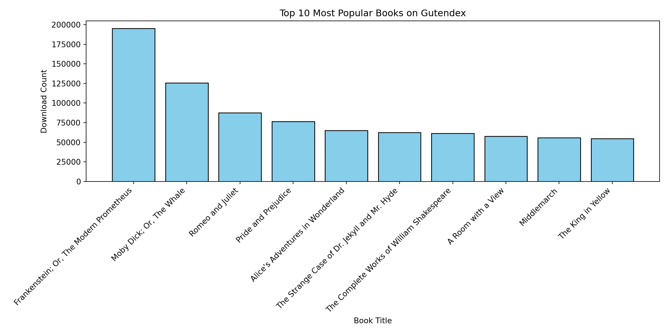
Case Study: Popularity of Books
- I want to demonstrate structuring data using a case study explaining the popularity of books on the basis of the (demographic) characteristics of their main characters.
- Source: Gutendex, an archive of books in the public domain (mainly written <1950).
- These books come with some metadata, including:
- Popularity (our dependent variable): no. of downloads on Gutendex
- A summary and the actual text of the book (which we will use to extract characteristics of the main characters)
Step 1: Extract and Clean Data
- Extracting the data from the API can be done using the following script:
- The script and the output DataFrame are also available online. 1
import requests
import polars as pl
import time

def fetch_gutendex_books(num_pages=100):
    base_url = "https://gutendex.com/books/"
    all_books = []

    # We use a session for connection pooling (more efficient for multiple requests)
    with requests.Session() as session:
        print(f"Starting to fetch {num_pages} pages...")

        for page in range(1, num_pages + 1):
            try:
                # Construct the URL with query parameters
                url = f"{base_url}?page={page}&topic=literature"

                response = session.get(url, timeout=10)
                response.raise_for_status() # Raise error for 404/500 codes

                data = response.json()

                # The actual book data is usually inside the 'results' key
                if 'results' in data:
                    all_books.extend(data['results'])

                print(f"Fetched page {page}/{num_pages}", end='\r')

                # Be polite to the API to avoid being banned
                time.sleep(2)

            except requests.exceptions.RequestException as e:
                print(f"\nError fetching page {page}: {e}")
                # Optional: break or continue depending on desired behavior
                continue

    print(f"\nParsing {len(all_books)} books into Polars DataFrame...")

    # Create DataFrame once from the list of dicts (Most efficient method)
    # infer_schema_length=None ensures Polars scans all rows to determine types correctly
    df = pl.DataFrame(all_books, infer_schema_length=None)

    return df

df = fetch_gutendex_books(50)
df_processed = (
    df
    # 0. Explode the summaries
    .explode(['summaries'])

    # 1. Keep only the first summary for each ID
    .unique(subset=["id"], keep="first")

    # 2. Overwrite 'authors' column with just the first author (Struct)
    .with_columns(
        pl.col("authors").list.first()
    )

    # 3. Unnest the struct fields into top-level columns
    # (This will likely create columns like 'name', 'birth_year', 'death_year')
    .unnest("authors")
)

#df_processed.write_parquet('books_processed.parquet')
#df_processed.select(['id', 'title', 'summaries', 'download_count']).write_csv("books_processed.csv", separator="\t")Popularity and Example Summaries
import polars as pl
import textwrap

print(textwrap.fill(df_processed['summaries'][0], 100))
## "Black Beauty" by Anna Sewell is a novel written in the late 19th century. The story is told from
## the perspective of a horse named Black Beauty, who recounts his experiences growing up on a farm,
## the trials he faces as he is sold into various homes, and the treatment he receives from different
## owners. The narrative touches on themes of animal welfare, kindness to creatures, and the importance
## of humane treatment.  At the start of the book, we are introduced to Black Beauty's early life in a
## peaceful meadow, where he lives with his mother, Duchess. He is fondly raised by a kind master and
## learns valuable lessons about good behavior from his mother. As he matures, the story unfolds to
## include his experiences with other horses, the harsh realities of training and harnessing, and the
## contrasting environments in which he lives – some nurturing, and others cruel. The opening chapters
## set the tone for a deeper exploration of social issues regarding the treatment of horses and the
## relationships they develop with humans. (This is an automatically generated summary.)

print(textwrap.fill(df_processed['summaries'][13], 100))
## "A Key to Uncle Tom's Cabin" by Harriet Beecher Stowe is a historical account written in the
## mid-19th century. The book serves as a companion piece to Stowe's famous novel "Uncle Tom's Cabin,"
## providing factual evidence, documents, and corroborative statements to verify the realities of
## slavery depicted in the fictional narrative. It aims to draw attention to the moral and ethical
## implications of slavery, evoking a serious contemplation of a deeply troubling institution.  The
## opening of "A Key to Uncle Tom's Cabin" begins with a preface wherein Stowe openly shares her
## struggle in writing this non-fiction work, emphasizing that slavery is an intrinsically dreadful
## subject. She notes that her task has expanded beyond her original intent, driven by the need to
## confront the painful truths surrounding slavery as a moral question. The first chapter focuses on
## various dynamics of the slave trade, illustrated through characters such as Mr. Haley, a slave
## trader, shedding light on the grim realities faced by individuals caught in this trade. Stowe
## underscores that the depictions in "Uncle Tom's Cabin," while fictionalized, are based on real
## events and sentiments, thus legitimizing the emotional and physical toll inflicted upon those
## ensnared in slavery. (This is an automatically generated summary.)
Step 2: Providing a pydantic Scheme
- Now, we create a
pydanticscheme that allows us to identify the characteristics of the main character(s) out of the summaries:
from pydantic import BaseModel, Field
from typing import List, Literal, Optional

class MainCharacter(BaseModel):
    species: Optional[str] = Field(
        default=None,
        description="The biological species or entity type of the character (e.g., Human, Elf, Robot)."
    )

    gender: Optional[Literal["Male", "Female"]] = Field(
        default=None,
        description="The biological sex or gender identity of the character."
    )

    age: Optional[Literal["Child", "Young Adult", "Adult", "Old Person"]] = Field(
        default=None,
        description="The approximate life stage or age category of the character."
    )

    moral_classification: Optional[Literal["Good", "Neutral", "Evil"]] = Field(
        default=None,
        description="The ethical alignment or moral compass of the character."
    )

class SummaryAnalysis(BaseModel):
    characters: List[MainCharacter] = Field(
        default_factory=list,
        description="A list of main characters found in the summary. Returns an empty list if none are found."
    )
Step 3: Feeding the Data and Structure to LLM
- Next, we pass all of the ~1500 summaries to GPT and extract the obtained data.
- The .csv output of this is also available online.
- In Python, this might take some time since you have to use batch processing.
import chatlas as ctl
from pydantic import BaseModel, Field
import polars as pl

chat = ctl.ChatOpenAI(model='gpt-4.1')
prompts = [summary for summary in df_processed['summaries']]
out = ctl.batch_chat_structured(chat, prompts, 'state.json', SummaryAnalysis)

# Put in Data.Frame
final_df = pl.DataFrame([
    {"id": i, "tmp": [c.model_dump() for c in x.characters] or [None]}
    for i, x in zip(df_processed['id'], out)
]).explode("tmp").unnest("tmp")

#final_df.write_csv("summaries_processed.csv")
Defining Data Structure
# R doesn't need a pydantic scheme - it can be defined on the spot here
main_character <- type_object(
    species = type_string(
        "The biological species or entity type of the character (e.g., Human, Elf, Robot).",
        required=FALSE),
    gender = type_enum(c("Male", "Female"),
        "The biological sex or gender identity of the character.",
        required=FALSE),
    age = type_enum(c("Child", "Young Adult", "Adult", "Old Person"),
        "The approximate life stage or age category of the character.",
        required=FALSE),
    moral_classification = type_enum(c("Good", "Neutral", "Evil"),
        "The ethical alignment or moral compass of the character.",
        required=FALSE)
        )

list_of_main_characters <- type_array(
    main_character,
    "List of all main characters mentioned in this text.",
    required=FALSE)
Data Processing
data_processed <- read_delim("books_processed.csv")
prompts <- as.list(
    data_processed$summaries
)

chat <- chat_openai(model="gpt-4.1")
out <- parallel_chat_structured(chat, prompts, type = list_of_main_characters)

# Post-processing into data.frame
final_df <- tibble(
  id = data_processed$id,
  data = out
) |>
  unnest(data, keep_empty = TRUE)

write_csv2(final_df, "summaries_processed.csv")
Step 4: Econometric analysis
- There are a number of ways to do this in a better way than what I am about to do (Random Forests, Neural Networks), but I will just briefly analyze the data using linear regression.
- We want to know whether the amount of main characters plays a role in predicting its popularity.
- We want to know whether the gender balance, age, or moral classification of the main characters plays a role.
- Data looks like this:1
Data Wrangling
summaries <- read_delim('summaries_processed.csv')
books_processed <- read_delim('books_processed.csv')
variables <- summaries |>
    group_by(id) |>
    summarize(
        no_of_protagonists = n(),
        male_ratio = mean(gender == "Male"),
        young_ratio = mean(age == "Young Adult"),
        goodbad = if_else(is.element("Evil", moral_classification), 1, 0))

analysis_df <- books_processed |>
    left_join(variables, by = 'id')

head(analysis_df, 3)
# A tibble: 3 × 8
id title summaries download_count no_of_protagonists male_ratio young_ratio
<dbl> <chr> <chr> <dbl> <int> <dbl> <dbl>
1 271 Blac… "\"Black… 5104 2 0.5 0.5
2 23997 Euge… "\"Eugen… 4794 2 1 1
3 155 The … "\"The M… 3125 2 1 0
# ℹ 1 more variable: goodbad <dbl>Step 4: Econometric Analysis [2]
- The number of protagonists and good vs. bad stories seem to be associated with more popularity.
| (1) | (2) | (3) | (4) | (5) | |
|---|---|---|---|---|---|
| + p < 0.1, * p < 0.05, ** p < 0.01, *** p < 0.001 | |||||
| (Intercept) | 7.784*** | 7.850*** | 7.837*** | 7.751*** | 7.814*** |
| (0.021) | (0.067) | (0.027) | (0.022) | (0.074) | |
| poly(no_of_protagonists, 2)1 | 3.957*** | 2.619** | |||
| (0.801) | (0.997) | ||||
| poly(no_of_protagonists, 2)2 | -2.367*** | -1.662*** | |||
| (0.427) | (0.467) | ||||
| male_ratio | -0.045 | -0.017 | |||
| (0.082) | (0.086) | ||||
| young_ratio | -0.095 | -0.090 | |||
| (0.068) | (0.069) | ||||
| goodbad | 0.252*** | 0.152* | |||
| (0.069) | (0.075) | ||||
| Num.Obs. | 1536 | 1369 | 1369 | 1536 | 1369 |
Conclusion
Conclusion
- Good project management is extremely important for your workflow.
- It can often determine the success or failure of a project.
- You will know when you work with somebody with a bad workflow (most likely you already know this).
- Hopefully I’ve gave a good example in the project about extracting structured data with LLM’s.
- As you have seen, extracting structured data is really straightforward thanks to a couple of really nice libraries,
pydanticandchatlasin Python, andellmerin R.
![]()
Project Organization and Structured Data with LLMs