Change of basis and a change of perspective
A location can be described using different directions and different units of distance. A point four metres east and two metres north of a fixed origin, for example, can also be reached by combining an eastward step with a diagonal step. The destination remains the same, while the numbers describing the route depend on the steps available. A change of basis formalizes this relationship.
The distinction between a vector and its coordinates is central to this idea. A vector describes a displacement, with a direction and a length. Its coordinates record how much of each chosen reference vector is required to produce that displacement. Changing the reference vectors changes the coordinates, even when the displacement remains fixed.
This post develops the distinction using a two-dimensional example. It first introduces bases and derives a matrix that converts between coordinates. It then explains matrix multiplication through its columns and rows, shows how a matrix can be recovered from observations, and connects the choice of basis to eigenvectors. The calculations require only multiplication, addition, and the solution of two simultaneous equations.
Vectors, bases, and coordinates
Consider a flat surface with a fixed origin. Distances are measured in metres, with east as the horizontal direction and north as the vertical direction. The standard basis consists of two vectors,
\[ e_1=\begin{pmatrix}1\\0\end{pmatrix}, \qquad e_2=\begin{pmatrix}0\\1\end{pmatrix}. \]
The first vector represents a displacement of one metre east; the second represents one metre north. The vector \(x\) pointing four metres east and two metres north can therefore be written as
\[ x=4e_1+2e_2=\begin{pmatrix}4\\2\end{pmatrix}. \]
A linear combination is a sum of vectors multiplied by numbers, such as \(4e_1+2e_2\). A basis is a collection of vectors that expresses every vector in the space as exactly one linear combination. In two dimensions, any two vectors pointing along different lines form a basis. They need not be perpendicular or have length one. Two vectors along the same line would fail because their combinations could never leave that line.
Now consider the alternative basis
\[ b_1=\begin{pmatrix}2\\0\end{pmatrix}, \qquad b_2=\begin{pmatrix}1\\1\end{pmatrix}. \]
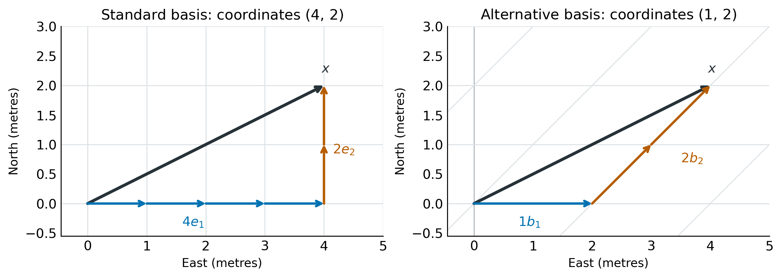
One step along \(b_1\) covers two metres east. One step along \(b_2\) covers one metre east and one metre north. The same displacement \(x\) is obtained with one step along \(b_1\) and two along \(b_2\):
\[ x=1b_1+2b_2 =\begin{pmatrix}2\\0\end{pmatrix} +2\begin{pmatrix}1\\1\end{pmatrix} =\begin{pmatrix}4\\2\end{pmatrix}. \]
The notation \([x]_B\) denotes the coordinates of \(x\) in this alternative basis. Thus \(x=(4,2)^T\) in standard coordinates, whereas \([x]_B=(1,2)^T\). The superscript \(T\) denotes transposition: writing \((4,2)^T\) turns a horizontal pair into a column. The two pairs of coordinates describe the same arrow, as shown in Figure 1.
Both descriptions use the same origin. Moving the origin would introduce an additional translation. A change of basis alone changes the directions or scales used to measure a displacement; it keeps the origin fixed.
Converting between coordinate systems
The alternative basis vectors can be collected as the columns of a matrix:
\[ B=\begin{pmatrix}|&|\\b_1&b_2\\|&|\end{pmatrix} =\begin{pmatrix}2&1\\0&1\end{pmatrix}. \]
Multiplying \(B\) by alternative coordinates reconstructs the vector in standard coordinates. In the example,
\[ x=B[x]_B =\begin{pmatrix}2&1\\0&1\end{pmatrix} \begin{pmatrix}1\\2\end{pmatrix} =\begin{pmatrix}4\\2\end{pmatrix}. \]
The direction of this conversion matters. Since the columns of \(B\) contain the new basis vectors expressed in standard coordinates, \(B\) converts from the alternative basis to the standard basis. To convert in the other direction, the equation must be solved for \([x]_B\).
This can be done without first knowing a formula for a matrix inverse. Let the unknown coordinates be \(c_1\) and \(c_2\). The equation \(x=c_1b_1+c_2b_2\) gives one equation for each standard coordinate:
\[ \begin{aligned} 4&=2c_1+c_2,\\ 2&=c_2. \end{aligned} \]
The second equation gives \(c_2=2\), and substituting this into the first gives \(c_1=1\). For an arbitrary vector \(x=(x_1,x_2)^T\), the same calculation gives \(c_2=x_2\) and \(c_1=(x_1-x_2)/2\). These two rules can themselves be written as a matrix:
\[ [x]_B=Mx, \qquad M=B^{-1}=\begin{pmatrix}1/2&-1/2\\0&1\end{pmatrix}. \]
The inverse \(B^{-1}\) reverses the operation performed by \(B\). In particular, \(B^{-1}B=I\), where the identity matrix \(I\) leaves every vector unchanged. A basis matrix has an inverse because every vector has a unique set of coordinates in that basis.
The same reasoning applies when neither basis is standard. If the columns of \(C\) contain the source basis vectors and the columns of \(B\) contain the target basis vectors, all expressed in standard coordinates, then
\[ x=C[x]_C=B[x]_B \qquad\Longrightarrow\qquad [x]_B=B^{-1}C[x]_C. \]
Read from right to left, \(C\) first reconstructs the vector from its source coordinates, and \(B^{-1}\) then expresses it in the target basis. The change of basis matrix is therefore \(B^{-1}C\). This formula also applies in three or more dimensions.
Reading a matrix by its columns and rows
The columns of a matrix describe the output associated with each unit of input. Multiplying \(M\) by \(e_1=(1,0)^T\) selects its first column; multiplying it by \(e_2=(0,1)^T\) selects its second. Here those columns contain the alternative coordinates of the two standard basis vectors:
\[ [e_1]_B=\begin{pmatrix}1/2\\0\end{pmatrix}, \qquad [e_2]_B=\begin{pmatrix}-1/2\\1\end{pmatrix}. \]
The first result says that half a \(b_1\) step produces one metre east. The second says that one \(b_2\) step combined with half a \(b_1\) step backwards produces one metre north. Negative coordinates therefore have a direct interpretation: they require movement opposite to the corresponding basis vector.
Since \(x=4e_1+2e_2\), its alternative coordinates are four times the first column plus twice the second:
\[ Mx =4\begin{pmatrix}1/2\\0\end{pmatrix} +2\begin{pmatrix}-1/2\\1\end{pmatrix} =\begin{pmatrix}1\\2\end{pmatrix}. \]
Reading the product by rows gives the same result. Each row produces one output coordinate by multiplying corresponding entries and adding them:
\[ Mx =\begin{pmatrix} \tfrac12\cdot4-\tfrac12\cdot2\\ 0\cdot4+1\cdot2 \end{pmatrix} =\begin{pmatrix}1\\2\end{pmatrix}. \]
This multiply-and-add operation is the dot product, also called the Euclidean inner product. For two vectors \(w=(w_1,w_2)^T\) and \(x=(x_1,x_2)^T\), it is \(w^Tx=w_1x_1+w_2x_2\). Each row of a matrix can be read as a dot product that extracts one number from the input.
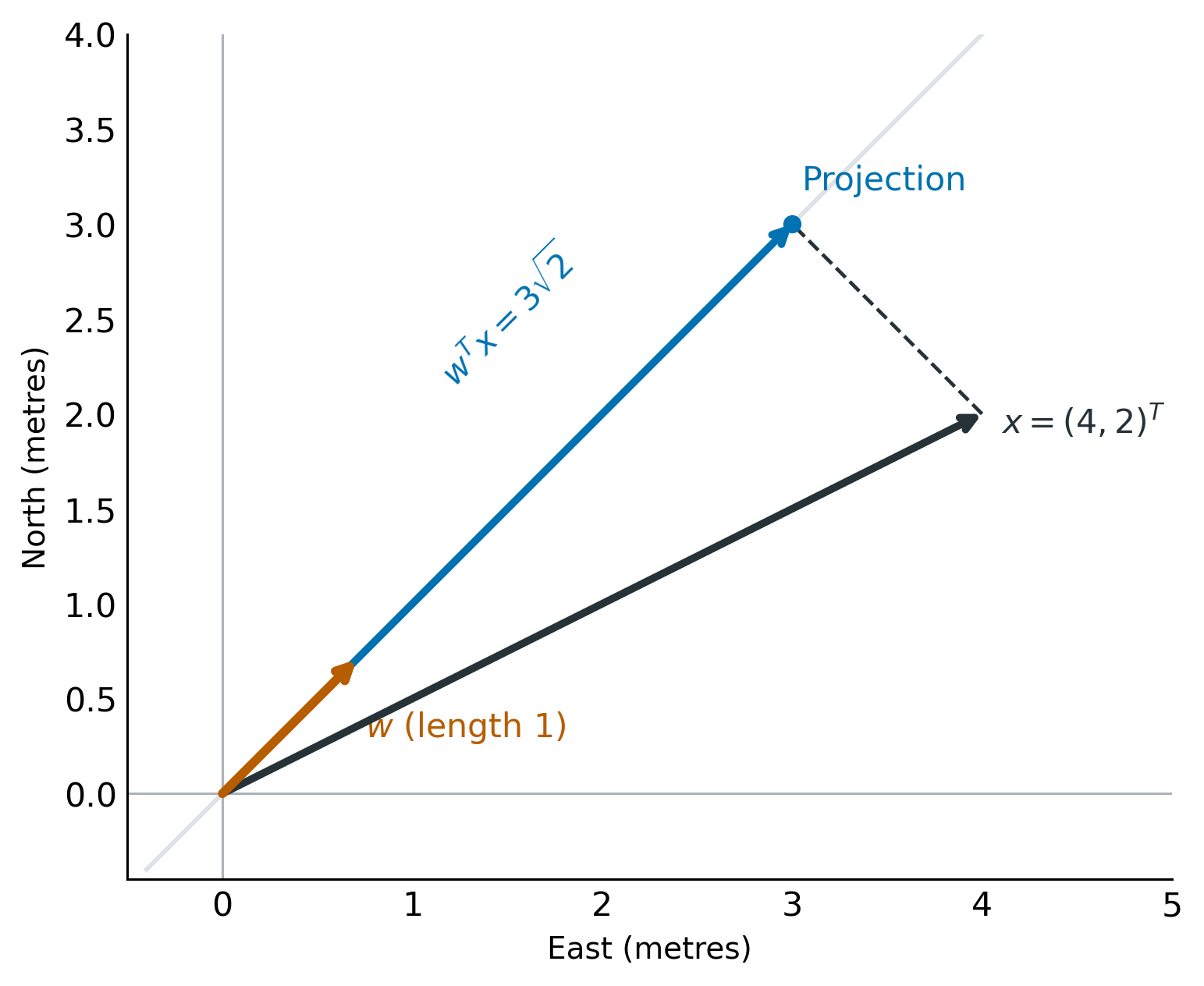
When \(w\) has length one, the dot product has a geometric interpretation: \(w^Tx\) is the signed length of the perpendicular projection of \(x\) onto the line in direction \(w\). The projection is the point on that line closest to the endpoint of \(x\). Its length is positive in the direction of \(w\) and negative in the opposite direction. Figure 2 illustrates this for \(w=(1,1)^T/\sqrt{2}\).
However, the rows of a change of basis matrix need not be unit vectors, or even point along the corresponding basis vectors. In this example, the first row of \(M\) is \((1/2,-1/2)\), although \(b_1\) points east. It subtracts the eastward movement already supplied by the diagonal steps before counting the remaining \(b_1\) steps. Coordinates coincide with dot products against the basis vectors when those vectors are perpendicular and each has length one, a basis called orthonormal. For a general basis, the inverse matrix supplies the appropriate coordinate rules.
Changing coordinates and transforming vectors
A matrix can also represent an operation that changes a vector while keeping the coordinate system fixed. These two uses of matrices share the same multiplication rules, but their interpretation depends on what the input and output coordinates describe. In the equation \(x=B[x]_B\), the input and output represent the same vector in different bases. In the equation \(y=Bx\), with both \(x\) and \(y\) expressed in the standard basis, the matrix defines a transformation of the vector itself.
For example, applying \(B\) to the standard coordinates \((4,2)^T\) gives
\[ y=Bx =\begin{pmatrix}2&1\\0&1\end{pmatrix} \begin{pmatrix}4\\2\end{pmatrix} =\begin{pmatrix}10\\2\end{pmatrix}. \]
The endpoint has now moved from \((4,2)\) to \((10,2)\). Under this interpretation, the first column of \(B\) gives the image of \(e_1\) and the second gives the image of \(e_2\). Applying the same operation to a whole grid produces the deformation in Figure 3.
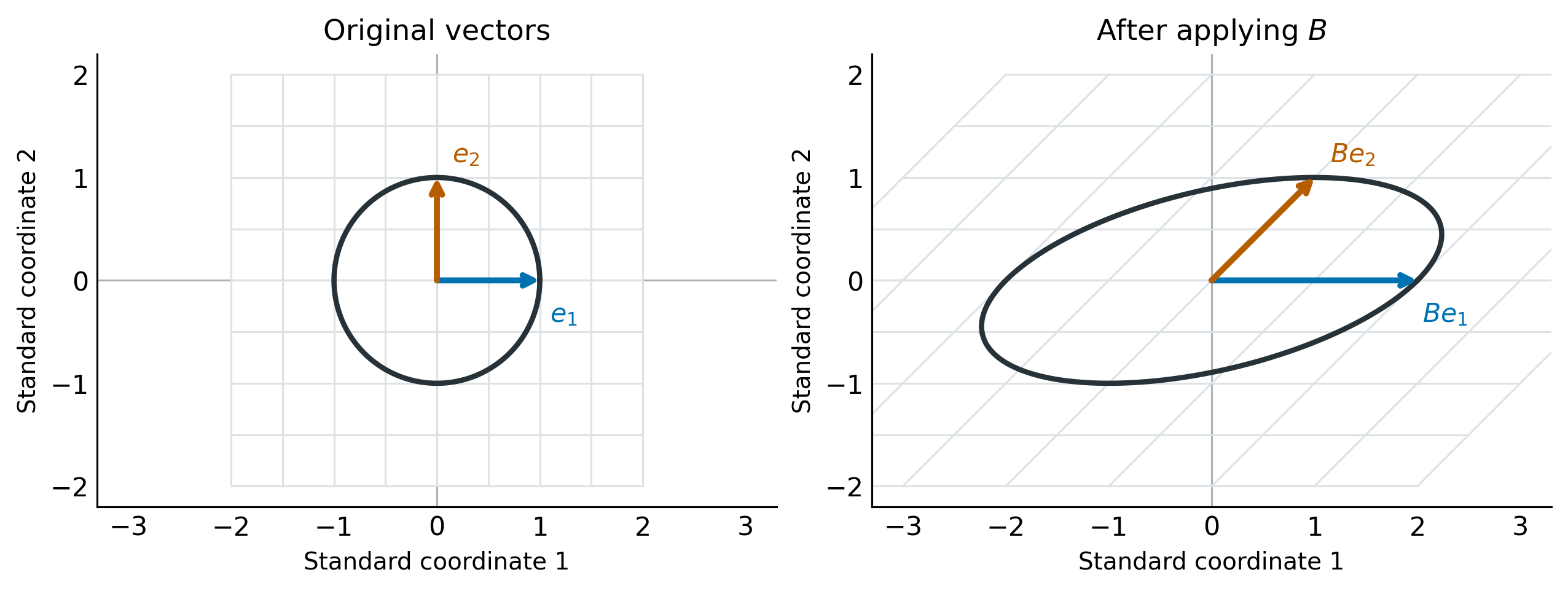
An operation represented by a matrix is linear: it respects addition and multiplication by a scalar. In symbols, \(B(u+v)=Bu+Bv\) and \(B(cu)=cBu\), where \(c\) is a number. These properties explain why knowing the images of the basis vectors determines the image of every vector. They also imply that the origin stays fixed. For an invertible matrix such as \(B\), straight lines remain straight and parallel lines remain parallel.
The circle in the figure consists of all vectors of length one. Its image under an invertible linear transformation in two dimensions is an ellipse. The longest and shortest radii of that ellipse measure the largest and smallest output lengths attainable from a unit input. These lengths are the singular values of the matrix. The singular value decomposition identifies the corresponding input and output directions. This interpretation uses ordinary Euclidean lengths in orthonormal coordinates; comparing coordinate lengths across arbitrary bases does not by itself measure a physical stretch. A singular matrix can collapse a circle to a line segment or a point, but such a matrix cannot convert between two bases because the conversion must be reversible.
Recovering a matrix from observations
Sometimes the basis vectors are unknown, but the coordinates of several vectors are observed in both systems. In two dimensions, two independent vectors suffice to identify a change of basis matrix. Independence here means that neither vector is a multiple of the other, so their combinations cover the plane.
Suppose the observed standard coordinates are \((2,0)^T\) and \((4,2)^T\), and their corresponding alternative coordinates are \((1,0)^T\) and \((1,2)^T\). Collecting each pair as columns gives
\[ X=\begin{pmatrix}2&4\\0&2\end{pmatrix}, \qquad Y=\begin{pmatrix}1&1\\0&2\end{pmatrix}. \]
The equation \(Y=MX\) states that the same unknown matrix \(M\) converts each column of \(X\) into the corresponding column of \(Y\). Multiplying on the right by \(X^{-1}\) gives
\[ M=YX^{-1} =\begin{pmatrix}1&1\\0&2\end{pmatrix} \begin{pmatrix}1/2&-1\\0&1/2\end{pmatrix} =\begin{pmatrix}1/2&-1/2\\0&1\end{pmatrix}. \]
This recovers the conversion matrix derived earlier. The order of multiplication matters: \(X^{-1}\) must appear on the right because it cancels the \(X\) on the right of \(M\). In three dimensions, the corresponding calculation requires three independent vectors. Three observations confined to a plane through the origin would leave the transformation outside that plane undetermined.
The calculation assumes exact observations generated by one linear map. With measurement error, a single matrix may fail to match every observed pair. Estimating a matrix that approximately fits the observations is then a separate problem, commonly addressed by least squares.
Eigenvectors and the choice of basis
A suitable basis can simplify the description of a linear transformation. Consider a new transformation, represented in standard coordinates by
\[ L=\begin{pmatrix}2&1\\1&2\end{pmatrix}. \]
For most vectors, \(L\) changes both length and direction. For example, it sends \((1,0)^T\) to \((2,1)^T\). However, the two diagonal directions behave differently:
\[ L\begin{pmatrix}1\\1\end{pmatrix} =\begin{pmatrix}3\\3\end{pmatrix} =3\begin{pmatrix}1\\1\end{pmatrix}, \qquad L\begin{pmatrix}1\\-1\end{pmatrix} =\begin{pmatrix}1\\-1\end{pmatrix}. \]
A nonzero vector \(v\) satisfying \(Lv=\lambda v\) is an eigenvector, and the number \(\lambda\) is its eigenvalue. For real eigenvectors, this means that the transformed vector stays on the same line through the origin. Here the direction \((1,1)^T\) is stretched by a factor of three, while \((1,-1)^T\) is unchanged. A negative eigenvalue would reverse the direction as well as scale the length, and an eigenvalue of zero would send the vector to the origin.
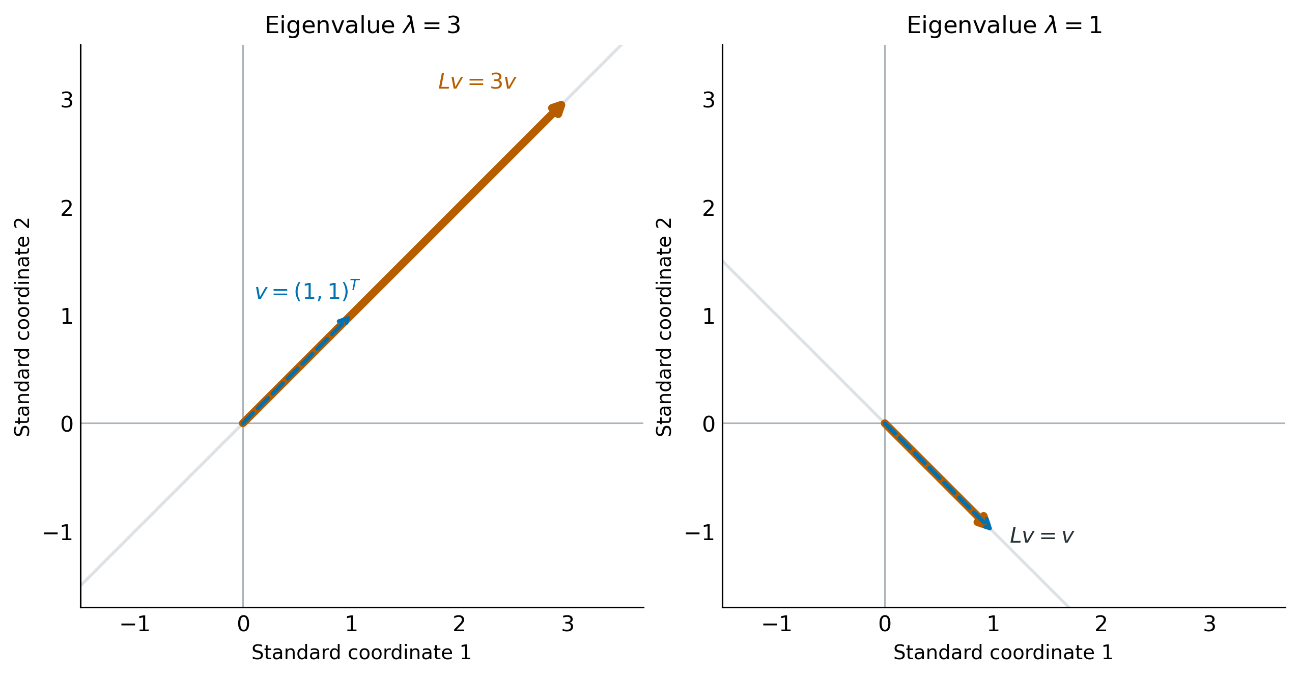
Every nonzero multiple of an eigenvector has the same eigenvalue: \(L(cv)=cLv=\lambda(cv)\). All vectors satisfying \(Lv=\lambda v\), including the zero vector, form the eigenspace for \(\lambda\). The zero vector belongs to the eigenspace but is excluded from the definition of an eigenvector. For this matrix, the two eigenspaces are the diagonal lines shown in Figure 4.
The two eigenvectors are independent, so they can serve as a basis. Let \(S\) collect them as columns. The matrix representing the transformation in this basis is
\[ S=\begin{pmatrix}1&1\\1&-1\end{pmatrix}, \qquad D=S^{-1}LS=\begin{pmatrix}3&0\\0&1\end{pmatrix}. \]
The expression \(S^{-1}LS\) describes three operations, read from right to left. First, \(S\) converts eigenvector coordinates to standard coordinates. Next, \(L\) applies the transformation. Finally, \(S^{-1}\) converts the result back to eigenvector coordinates. In this basis, the transformation multiplies the first coordinate by three and leaves the second unchanged. The off-diagonal zeros show that neither coordinate contributes to the other.
For a numerical check, the vector \(x=(4,2)^T\) has eigenvector coordinates \([x]_S=(3,1)^T\), because \(3(1,1)^T+(1,-1)^T=(4,2)^T\). Applying \(D\) produces \((9,1)^T\). Converting back gives \(9(1,1)^T+(1,-1)^T=(10,8)^T\), which is also the result of multiplying \(Lx\) directly.
Such a basis exists only when the transformation has enough independent eigenvectors in the number system being used. For example, a rotation of the plane by 90 degrees has no real eigenvectors, because every nonzero vector leaves its original line. A change of basis remains possible, but it cannot turn that rotation into independent scaling along real coordinate axes.
Conclusion
A change of basis expresses a fixed vector using a different set of reference vectors. Placing those reference vectors in the columns of \(B\) gives the reconstruction rule \(x=B[x]_B\); reversing that rule gives the coordinate conversion \([x]_B=B^{-1}x\). Reading a matrix by columns explains how it combines input directions, while reading it by rows explains how it calculates each output coordinate.
The choice of basis also affects how a linear transformation is represented. When independent eigenvectors form a basis, the transformation reduces to separate scaling operations in those coordinates. The example above turns the matrix \(L\) into the diagonal matrix with entries three and one, while preserving the underlying transformation.