Orthogonal bases, Gram–Schmidt, and QR decomposition
Introduction
Least squares asks for the point in the column space of a data matrix that is closest to an outcome vector. The normal equations express this condition in the original, usually non-orthogonal, columns of the matrix. QR decomposition instead constructs an orthonormal basis for the same column space. In that basis, projection and least squares reduce to dot products and triangular back-substitution.
Let \(X\in\mathbb{R}^{N\times k}\) be a matrix with \(N\geq k\) and full column rank \(k\). Its columns \(x_1,\ldots,x_k\in\mathbb{R}^N\) may be regressors, or variables measured for \(N\) observations. Full column rank means that no column is an exact linear combination of the preceding columns. This post first constructs an orthonormal basis from these columns using Gram–Schmidt, then writes the construction as a QR decomposition, and finally uses it to solve least squares.
Orthogonality makes coordinates simple
A collection of vectors \(q_1,\ldots,q_k\in\mathbb{R}^N\) is orthonormal when
\[ q_i^\top q_j= \begin{cases} 1 & \text{if }i=j,\\ 0 & \text{if }i\neq j. \end{cases} \]
Put these vectors in the \(N\times k\) matrix \(Q=(q_1,\ldots,q_k)\). The preceding conditions are exactly
\[ Q^\top Q=I_k. \]
The subscript matters. When \(N>k\), \(Q\) is rectangular, so \(QQ^\top\) is an \(N\times N\) matrix but cannot equal \(I_N\): the \(k\) columns span only a \(k\)-dimensional part of \(\mathbb{R}^N\).
Coordinates are properties of a representation, not of the vector itself. Let \(E=(e_1,\ldots,e_N)\) be the standard basis of \(\mathbb{R}^N\). The columns \(q_1,\ldots,q_k\) of \(Q\) are written in this standard basis, and they form the orthonormal basis \(\mathcal{Q}=(q_1,\ldots,q_k)\) of \(\operatorname{col}(Q)\). For a vector \(z\in\operatorname{col}(Q)\), write \([z]_E\in\mathbb{R}^N\) for its standard-coordinate column and \([z]_{\mathcal{Q}}\in\mathbb{R}^k\) for its coordinate column in the \(\mathcal{Q}\) basis. If \(a=[z]_{\mathcal{Q}}\), then
\[ z=\sum_{j=1}^k a_jq_j, \qquad [z]_E=Qa. \]
Thus \(Q\) converts coordinates from the \(\mathcal{Q}\) basis to the standard basis. Because \(Q^\top Q=I_k\), the reverse conversion is especially simple:
\[ Q^\top[z]_E=Q^\top Qa=a=[z]_{\mathcal{Q}}. \]
The \(j\)th coordinate in the \(\mathcal{Q}\) basis is therefore \(a_j=q_j^\top[z]_E\). This is the advantage of an orthonormal basis: each coordinate is one dot product with its basis vector.
For a complete orthonormal basis of \(\mathbb{R}^N\), \(Q\) is square and \(Q^\top Q=I_N\), so \(Q^\top=Q^{-1}\). This equality is the reason the transpose converts standard coordinates back to orthonormal-basis coordinates. In the reduced QR decomposition, \(Q\) is usually \(N\times k\) with \(N>k\), so it has no two-sided inverse. Its transpose is instead a left inverse on the column space: \(Q^\top Q=I_k\) and \(Q^\top[z]_E=[z]_{\mathcal{Q}}\) for every \(z\in\operatorname{col}(Q)\).
For comparison, let \(B=(b_1,\ldots,b_k)\) be a basis that is not orthonormal, with its columns also written in standard coordinates. The same vector satisfies \([z]_E=B[z]_{\mathcal{B}}\), but its coordinates must generally be obtained by solving a system:
\[ [z]_{\mathcal{B}}=B^{-1}[z]_E. \]
Multiplying by \(B^\top\) does not extract the coordinates, because the basis vectors are neither perpendicular nor necessarily of length one. The dot products \(b_j^\top[z]_E\) include contributions from the other basis directions.
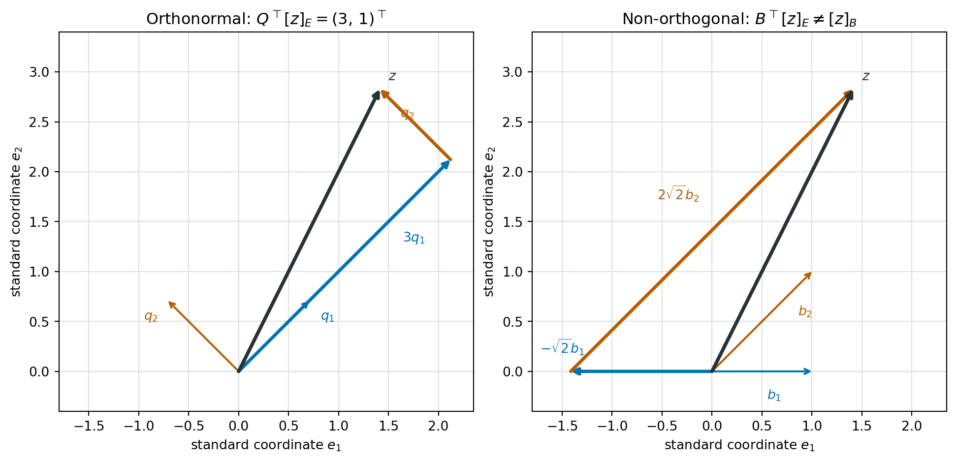
For example, take \(N=k=2\) and rotate the standard basis by \(45^\circ\):
\[ Q= \begin{pmatrix} 1/\sqrt{2} & -1/\sqrt{2}\\ 1/\sqrt{2} & 1/\sqrt{2} \end{pmatrix} =(q_1,q_2), \qquad [z]_{\mathcal{Q}}=a= \begin{pmatrix}3\\1\end{pmatrix}. \]
This specifies the coordinates, rather than a different vector: \([z]_{\mathcal{Q}}=(3,1)^\top\) and the same vector has standard coordinates
\[ [z]_E=Q[z]_{\mathcal{Q}} = \begin{pmatrix}\sqrt{2}\\2\sqrt{2}\end{pmatrix}. \]
The two coordinates in the \(\mathcal{Q}\) basis are recovered directly:
\[ Q^\top[z]_E= \begin{pmatrix} q_1^\top[z]_E\\q_2^\top[z]_E \end{pmatrix} = \begin{pmatrix}3\\1\end{pmatrix} =a. \]
Now use the non-orthogonal basis \(\mathcal{B}=(b_1,b_2)\), with \(b_1=(1,0)^\top\) and \(b_2=(1,1)^\top\), to represent this same \(z\). The figure shows that its basis coordinates are \([z]_{\mathcal{B}}=(-\sqrt{2},2\sqrt{2})^\top\). Its dot products with the non-orthogonal basis are instead \(B^\top[z]_E=(\sqrt{2},3\sqrt{2})^\top\), which are not its coordinates.
The two panels reach the same \(z\). The left panel permits coordinate recovery by two dot products. The right panel requires the inverse of the basis matrix, even though both bases span the same plane.
Classical Gram–Schmidt
Gram–Schmidt replaces the original independent columns \(x_1,\ldots,x_k\) by orthonormal columns that span exactly the same subspaces at every stage. Begin with the first column. It has no earlier direction to remove, so set
\[ r_{11}=\lVert x_1\rVert_2, \qquad q_1=\frac{x_1}{r_{11}}. \]
Here \(r_{11}>0\) because full column rank implies \(x_1\neq0\). The vector \(q_1\) has length one and spans the same line as \(x_1\).
For a later column \(x_j\), \(j=2,\ldots,k\), first find its component in each earlier orthonormal direction:
\[ r_{ij}=q_i^\top x_j, \qquad i=1,\ldots,j-1. \]
The projection of \(x_j\) onto the span of \(q_1,\ldots,q_{j-1}\) is therefore \(\sum_{i=1}^{j-1}r_{ij}q_i\). Subtracting it leaves
\[ v_j=x_j-\sum_{i=1}^{j-1}r_{ij}q_i. \]
This remainder is perpendicular to every earlier \(q_\ell\). To see this, take its dot product with \(q_\ell\), where \(\ell<j\):
\[ q_\ell^\top v_j =q_\ell^\top x_j- \sum_{i=1}^{j-1}(q_i^\top x_j)(q_\ell^\top q_i) =q_\ell^\top x_j-q_\ell^\top x_j=0. \]
All terms in the sum disappear except \(i=\ell\), since the earlier \(q_i\) are orthonormal. Full column rank ensures that \(v_j\neq0\): if it were zero, \(x_j\) would be a combination of earlier columns. We can consequently normalize it,
\[ r_{jj}=\lVert v_j\rVert_2, \qquad q_j=\frac{v_j}{r_{jj}}. \]
This procedure is called classical Gram–Schmidt. It identifies all the old components of \(x_j\) using the original column, subtracts them together, and then normalizes what remains.
QR decomposition
For each column \(j\), Gram–Schmidt first separates \(x_j\) into its projection on the earlier orthonormal directions and the perpendicular remainder:
\[ x_j=\sum_{i=1}^{j-1}r_{ij}q_i+v_j. \]
The normalization step gives \(v_j=r_{jj}q_j\). Substituting this expression for the remainder gives
\[ x_j=r_{1j}q_1+\cdots+r_{j-1,j}q_{j-1}+r_{jj}q_j. \]
There is no \(q_i\) term for \(i>j\). If \(R\in\mathbb{R}^{k\times k}\) has entries \(r_{ij}\) from these expressions, it is upper triangular:
\[ R= \begin{pmatrix} r_{11} & r_{12} & \cdots & r_{1k}\\ 0 & r_{22} & \cdots & r_{2k}\\ \vdots & \ddots & \ddots & \vdots\\ 0 & \cdots & 0 & r_{kk} \end{pmatrix}. \]
The columns that multiply the entries of \(R\) are collected in
\[ Q= \begin{pmatrix} \vert & \vert & & \vert\\ q_1 & q_2 & \cdots & q_k\\ \vert & \vert & & \vert \end{pmatrix}_{N\times k}. \]
Stacking the \(k\) column identities produces the reduced QR factorization
\[ \underbrace{X}_{N\times k} = \underbrace{Q}_{N\times k} \underbrace{R}_{k\times k}, \qquad Q^\top Q=I_k. \]
The word reduced distinguishes this factorization from a full QR factorization, which adds \(N-k\) orthonormal columns to make an \(N\times N\) orthogonal matrix. The reduced form contains precisely the \(k\) directions needed for the column space of \(X\). Because each diagonal entry \(r_{jj}\) is positive, \(R\) is invertible. The factorization also shows that \(\operatorname{col}(X)=\operatorname{col}(Q)\): multiplication by an invertible \(R\) changes coordinates but does not change the set of attainable vectors.
Modified Gram–Schmidt
The preceding derivation uses exact arithmetic. On a computer, dot products and subtractions are rounded. When \(x_j\) is nearly in the span of the earlier columns, subtracting all of its projected components at once can leave a vector that is not quite orthogonal to those columns.
Modified Gram–Schmidt performs the same algebra in a different order. Start with working columns \(v_1=x_1,\ldots,v_k=x_k\). At step \(i\), normalize the current working column,
\[ r_{ii}=\lVert v_i\rVert_2, \qquad q_i=\frac{v_i}{r_{ii}}, \]
and then remove its component from every remaining working column:
\[ r_{ij}=q_i^\top v_j, \qquad v_j\leftarrow v_j-r_{ij}q_i, \qquad j=i+1,\ldots,k. \]
After step \(i\), each remaining \(v_j\) has had its \(q_i\) component removed before the next projection is calculated. In exact arithmetic, both algorithms produce the same \(Q\) and \(R\). With floating-point arithmetic, modified Gram–Schmidt normally preserves orthogonality better. Production QR routines for dense matrices often use Householder reflections, which are more robust still, but Gram–Schmidt exposes the geometric construction directly.
Least squares without the normal equations
Let \(y\in\mathbb{R}^N\) be an outcome vector. Least squares chooses \(\hat\beta\in\mathbb{R}^k\) to minimize
\[ \lVert y-X\beta\rVert_2^2 =\lVert y-QR\beta\rVert_2^2. \]
The vector \(QQ^\top y\) is the projection of \(y\) onto \(\operatorname{col}(Q)\). The remaining vector \((I_N-QQ^\top)y\) is orthogonal to that space. Hence the residual can be split into perpendicular pieces,
\[ y-QR\beta =Q(Q^\top y-R\beta)+(I_N-QQ^\top)y. \]
The first term lies in \(\operatorname{col}(Q)\) and the second is perpendicular to it. Pythagoras therefore gives
\[ \lVert y-QR\beta\rVert_2^2 =\lVert Q^\top y-R\beta\rVert_2^2 +\lVert(I_N-QQ^\top)y\rVert_2^2. \]
The second term cannot be changed by \(\beta\). The first reaches zero because \(R\) is invertible, so the least-squares coefficients solve
\[ R\hat\beta=Q^\top y. \]
This is a \(k\times k\) upper-triangular system. Its last equation determines \(\hat\beta_k\), after which the preceding equations determine \(\hat\beta_{k-1},\ldots,\hat\beta_1\). This procedure is called back-substitution. The fitted values and projection matrix are
\[ \hat y=X\hat\beta=QQ^\top y, \qquad P_X=QQ^\top. \]
The matrix \(P_X\) is symmetric because \((QQ^\top)^\top=QQ^\top\), and idempotent because \(P_X^2=Q(Q^\top Q)Q^\top=QQ^\top\). These are the defining algebraic properties of an orthogonal projection.
Conditioning and rank deficiency
The normal-equations route starts from \(X^\top X\hat\beta=X^\top y\). QR avoids forming \(X^\top X\). This distinction matters when columns of \(X\) are nearly dependent. In the Euclidean norm, the condition number of a full-column-rank matrix is
\[ \kappa_2(X)=\frac{\sigma_{\max}(X)}{\sigma_{\min}(X)}, \]
where the singular values describe the largest and smallest stretching caused by \(X\). A large value means that small perturbations in the data can cause large changes in the fitted coefficients. Since the singular values of \(X^\top X\) are \(\sigma_i(X)^2\),
\[ \kappa_2(X^\top X)=\kappa_2(X)^2. \]
Forming the normal equations therefore squares the numerical difficulty as well as the matrix. QR solves the equivalent least-squares problem while avoiding this amplification. It cannot remove genuine statistical uncertainty from nearly collinear regressors, but it avoids adding unnecessary numerical error.
If \(X\) is rank deficient, some \(v_j\) has zero length and the reduced \(N\times k\) QR construction above stops: the corresponding diagonal element of \(R\) is zero. Least-squares fitted values remain uniquely defined as the projection onto \(\operatorname{col}(X)\), but coefficients need not be unique. A pivoted QR decomposition can reveal the independent columns and numerical rank. The singular value decomposition gives a more general treatment: it identifies near-zero singular values and, through the pseudoinverse, selects the minimum-length coefficient vector among the least-squares solutions.
Conclusion
Gram–Schmidt constructs an orthonormal basis for the column space without changing that space. Collecting the resulting coordinate weights yields the reduced factorization \(X=QR\), in which least squares reduces to projection by \(QQ^\top\) and solution of an upper-triangular system. This avoids the numerical deterioration caused by forming \(X^\top X\), although it cannot resolve genuine near dependence in the data. When rank is deficient, pivoted QR or the singular value decomposition is needed to identify the directions the data determine.