Singular value decomposition
Introduction
Many economic datasets can be represented by a rectangular matrix. Let \(X\) contain \(N\) observations in its rows and \(k\) variables in its columns. A row might describe a worker, firm, municipality, or country. A column might record income, schooling, productivity, or employment. Even when \(k\) is large, much of the variation often moves along a smaller number of directions. Income, schooling, and productivity, for example, may share a common direction associated with economic development.
The singular value decomposition, or SVD, identifies these directions. For any real \(m\times n\) matrix \(A\), it produces three matrices such that
\[ A=U\Sigma V^\top. \]
The formula is compact, but it does not by itself convey what the three factors mean. The columns of \(V\) identify orthogonal directions among the inputs. The diagonal entries of \(\Sigma\) state how strongly \(A\) acts along each direction. The columns of \(U\) identify the corresponding directions among the outputs. Thus, the SVD describes a matrix by matching input directions to output directions and attaching a scale to every match.
The discussion below begins with a two-dimensional transformation because its geometry can be drawn. It then establishes the decomposition for every real rectangular matrix and applies it to a synthetic dataset with 160 observations and 4 economic variables. The final sections connect the same decomposition to principal components, low-rank approximation, least squares, and multicollinearity.
A matrix turns a circle into an ellipse
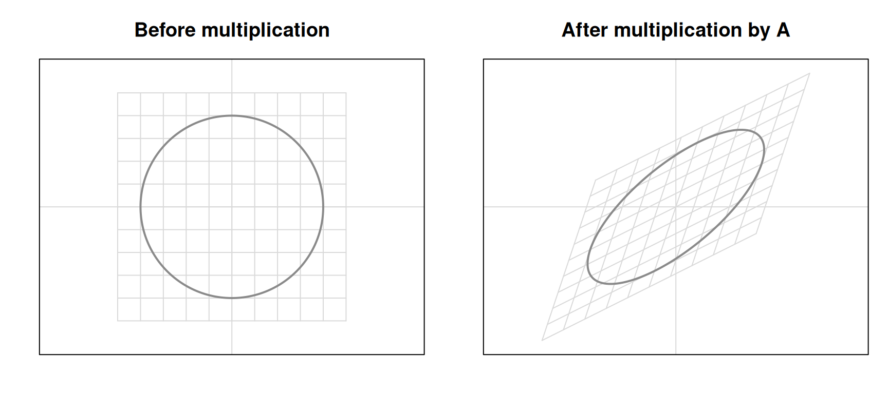
A matrix represents a linear transformation. In two dimensions, its action can be seen by applying it to a square grid and to the unit circle. The matrix used in Figure 1 is
\[ A= \begin{pmatrix} 2 & 0.5\\ 1 & 1.5 \end{pmatrix}. \]
Linearity rules out bending: \(A(x+y)=Ax+Ay\) and \(A(cx)=cAx\). The output therefore remains smooth and symmetric around the origin. More precisely, the image of the unit circle is an ellipse. If the matrix collapses one direction, the ellipse becomes a line segment or a point. In higher dimensions, the unit sphere becomes an ellipsoid inside the column space of \(A\).
An ellipse has perpendicular principal axes. Consequently, there are perpendicular input directions whose images point along those axes. Denote the input directions by \(v_1\) and \(v_2\), their output directions by \(u_1\) and \(u_2\), and the corresponding lengths by \(\sigma_1\) and \(\sigma_2\). They satisfy
\[ Av_1=\sigma_1u_1, \qquad Av_2=\sigma_2u_2. \]
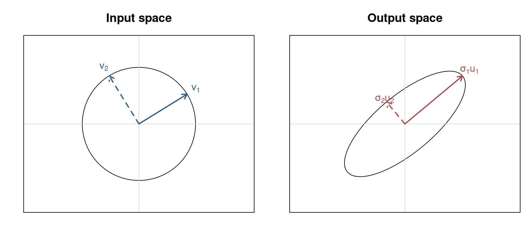
Figure 2 displays these matched directions on the unit circle and its image.
The directions \(v_j\) are the right singular vectors, the directions \(u_j\) are the left singular vectors, and the nonnegative numbers \(\sigma_j\) are the singular values. Singular values are conventionally ordered from largest to smallest. The first pair therefore describes the direction that \(A\) stretches most strongly.
Three simple operations
The factorization \(A=U\Sigma V^\top\) is read from right to left. The multiplication \(V^\top x\) measures the coordinates of \(x\) along the right singular vectors. The diagonal matrix \(\Sigma\) multiplies coordinate \(j\) by \(\sigma_j\). Finally, \(U\) rebuilds the output from the left singular vectors. Figure 3 applies these operations to the entire unit circle and to the two right singular vectors.
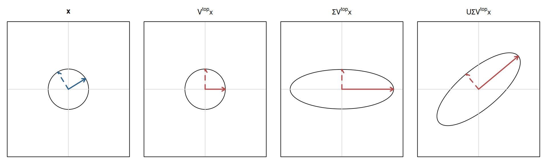
Orthogonal matrices such as \(V^\top\) and \(U\) preserve lengths and angles. In two dimensions they rotate or reflect the picture. All changes in length occur inside \(\Sigma\). This separation explains why singular values provide a direct measure of the strength of a transformation. A direction associated with a small singular value has little effect on the output, whereas a direction associated with a zero singular value disappears entirely.
For a general \(m\times n\) matrix, the full decomposition has the following dimensions.
| Object | Dimensions | Interpretation |
|---|---|---|
| \(V^\top\) | \(n\times n\) | Coordinates along orthogonal input directions |
| \(\Sigma\) | \(m\times n\) | Nonnegative scale attached to each matched direction |
| \(U\) | \(m\times m\) | Reconstruction along orthogonal output directions |
If \(r=\operatorname{rank}(A)\), only \(r\) singular values are positive. The thin SVD retains only these directions:
\[ A=U_rD_rV_r^\top, \]
where \(U_r\) is \(m\times r\), \(D_r\) is \(r\times r\), and \(V_r\) is \(n\times r\). This form contains the same information as the full decomposition without carrying bases for directions that contribute nothing to \(A\).
A matrix as a sum of layers
Matrix multiplication can also be read one singular direction at a time. Expanding the thin SVD gives
\[ A=\sigma_1u_1v_1^\top+\sigma_2u_2v_2^\top+\cdots+\sigma_ru_rv_r^\top. \]
Each outer product \(u_jv_j^\top\) is a rank-one matrix. Given an input \(x\), the scalar \(v_j^\top x\) measures its component along \(v_j\). The layer then multiplies this component by \(\sigma_j\) and places it along \(u_j\):
\[ \left(\sigma_ju_jv_j^\top\right)x =\sigma_j\left(v_j^\top x\right)u_j. \]
The two layers of the running \(2\times2\) example are shown separately in Figure 4. A rank-one transformation collapses the unit circle to a line segment. Adding the two layers restores the ellipse.
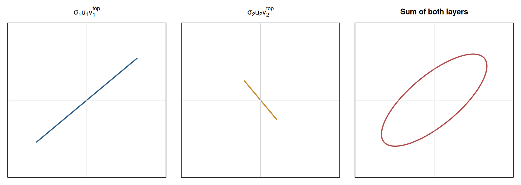
This representation also gives the rank of \(A\): it is the number of positive singular values. The right singular vectors associated with positive singular values span the row space, while those associated with zero singular values span the null space. The corresponding left singular vectors span the column space.
Why the decomposition exists for every real matrix
The geometric argument identifies the result in two dimensions, but it does not establish the decomposition in higher dimensions. A general proof follows from the spectral theorem for real symmetric matrices: if \(B=B^\top\), then \(B\) has an orthonormal basis of real eigenvectors and all its eigenvalues are real.
Let \(A\in\mathbb R^{m\times n}\) and consider \(A^\top A\). This is a real symmetric matrix because
\[ (A^\top A)^\top=A^\top A. \]
It is also positive semidefinite. For every \(x\in\mathbb R^n\),
\[ x^\top A^\top Ax=\lVert Ax\rVert^2\geq 0. \]
The spectral theorem therefore supplies an orthonormal basis \(v_1,\ldots,v_n\) and nonnegative eigenvalues \(\lambda_1\geq\cdots\geq\lambda_n\geq0\) satisfying
\[ A^\top Av_j=\lambda_jv_j. \]
Define \(\sigma_j=\sqrt{\lambda_j}\). Suppose first that \(\sigma_j>0\), and define
\[ u_j=\frac{Av_j}{\sigma_j}. \]
These vectors have unit length and are mutually orthogonal. Indeed,
\[ u_i^\top u_j =\frac{v_i^\top A^\top Av_j}{\sigma_i\sigma_j} =\frac{\lambda_jv_i^\top v_j}{\sigma_i\sigma_j} = \begin{cases} 1,&i=j,\\ 0,&i\neq j. \end{cases} \]
Let \(r\) be the number of positive singular values. The vectors \(u_1,\ldots,u_r\) can be completed to an orthonormal basis of \(\mathbb R^m\). Place this basis in the columns of \(U\), place the vectors \(v_1,\ldots,v_n\) in the columns of \(V\), and put the positive singular values on the diagonal of the \(m\times n\) matrix \(\Sigma\).
It remains to check the directions with zero singular values. If \(j>r\), then
\[ \lVert Av_j\rVert^2 =v_j^\top A^\top Av_j =\lambda_j =0, \]
so \(Av_j=0\). Consequently, \(A\) and \(U\Sigma V^\top\) agree on every basis vector \(v_j\): both send \(v_j\) to \(\sigma_ju_j\) when \(j\leq r\), and both send it to zero otherwise. Two linear transformations that agree on a basis are equal. Hence
\[ A=U\Sigma V^\top. \]
The proof uses only real matrices. It covers tall, wide, square, and rank-deficient matrices. The decomposition need not be unique. The signs of a pair \(u_j,v_j\) can be reversed together, and repeated singular values permit different orthonormal bases within the corresponding subspace. The singular values themselves are nevertheless fixed.
The same decomposition for a data table
Consider a data matrix \(X\in\mathbb R^{N\times k}\). The synthetic example contains four variables generated from two latent factors and independent noise. Each column is centered and divided by its sample standard deviation. This standardization prevents a variable from dominating merely because it is recorded in larger units. It also means that the covariance matrix below is the sample correlation matrix of the original variables.
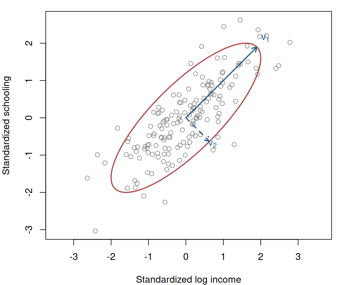
The two-variable view in Figure 5 shows the first connection between the SVD and a dataset. The observations form a point cloud. Its principal directions are the right singular vectors, and its standard deviations along those directions are \(d_j/\sqrt{N-1}\).
Write the thin SVD of the full data matrix as \(X=UDV^\top\). Its sample covariance matrix is
\[ S=\frac{X^\top X}{N-1} =V\frac{D^2}{N-1}V^\top. \]
The columns of \(V\) are therefore the eigenvectors of the covariance matrix. In principal component terminology, they are the component directions. Some software calls these vectors loadings, whereas other software reserves that term for coefficients scaled by the component standard deviations. The associated covariance eigenvalues are \(d_j^2/(N-1)\). This identity is the algebraic counterpart of the ellipse: \(V\) supplies its axes and \(D/\sqrt{N-1}\) supplies their lengths.
The coordinates of the observations along the new axes are obtained by projecting the rows of \(X\) onto \(V\):
\[ XV=UD. \]
Thus, \(UD\), rather than \(U\) alone, is the matrix of principal-component scores. The \(j\)th column records the location of every observation along component \(j\). Figure 6 shows the first two scores and the coefficients that define these directions from the original variables.
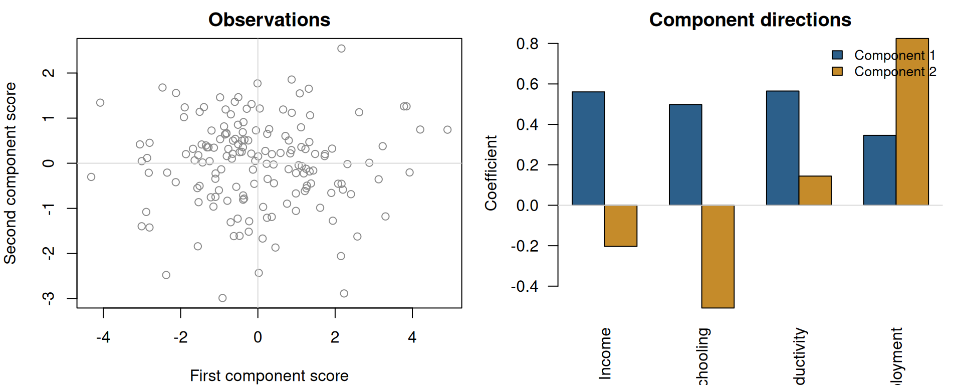
The first component assigns similar signs to income, schooling, productivity, and employment, reflecting their common latent factor in the simulated data. The second component distinguishes labour-market variation from the broader development direction. These interpretations are properties of this particular data-generating process, not general definitions of the first and second components.
Low-rank approximation
Ordering the singular values makes it possible to retain the strongest layers and discard the rest. The rank-\(q\) approximation is
\[ X_q=\sum_{j=1}^q d_ju_jv_j^\top. \]
The Eckart-Young theorem states that \(X_q\) minimizes the reconstruction error among all matrices of rank at most \(q\). Under the Frobenius norm,
\[ \min_{\operatorname{rank}(B)\leq q}\lVert X-B\rVert_F^2 =\lVert X-X_q\rVert_F^2 =\sum_{j=q+1}^r d_j^2. \]
Under the operator norm, the minimum error is \(d_{q+1}\). The result gives a precise meaning to the claim that small singular directions contain less of the matrix. Removing them loses less squared variation than removing any other collection of directions of the same dimension.
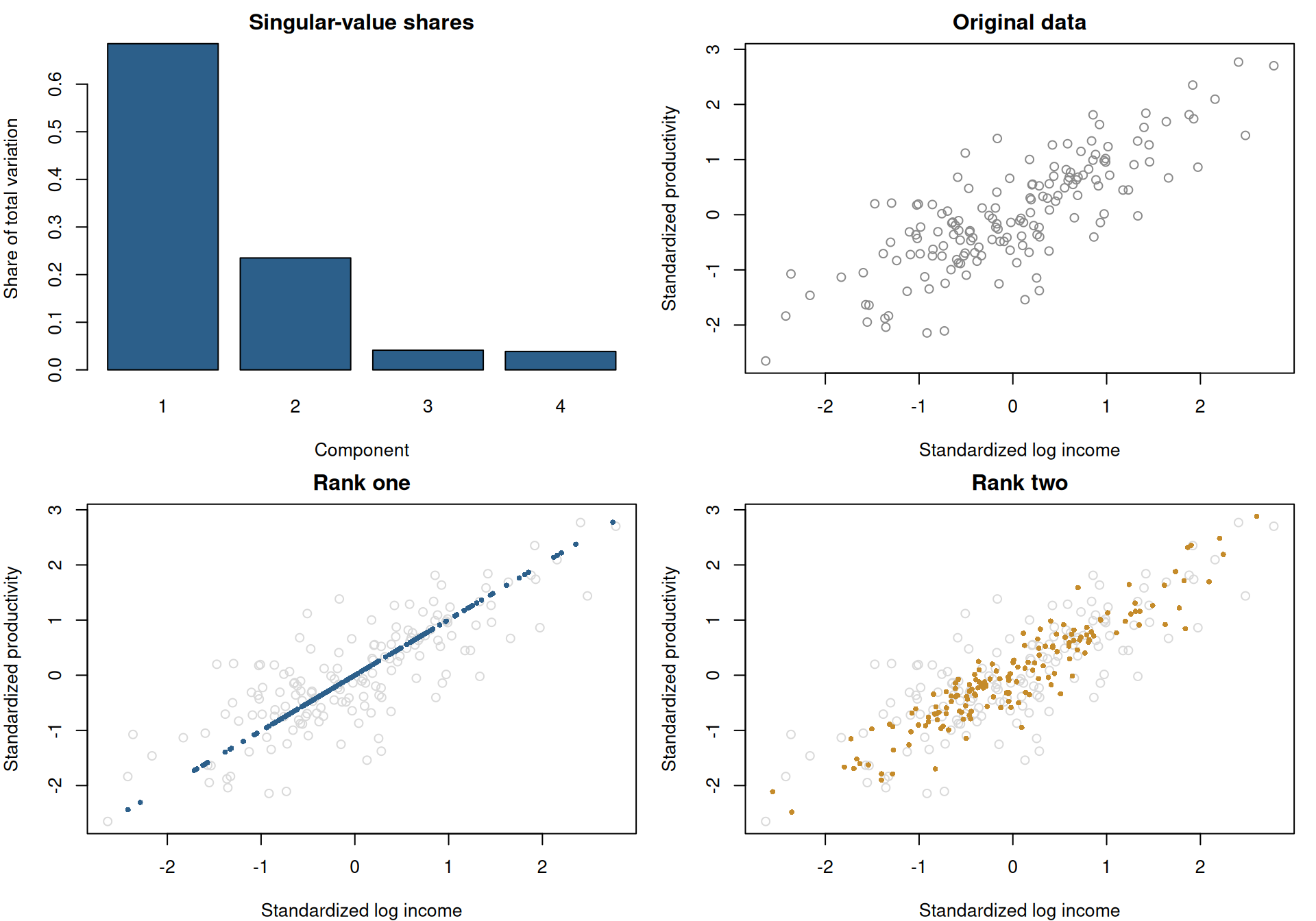
For this dataset, the first approximation places every observation on one line. The second allows a second independent direction and recovers most of the visible cloud. In empirical work, the appropriate rank cannot be selected from a picture alone. It depends on the purpose of the approximation, the amount of sampling noise, and the consequences of discarding variation.
Least squares and multicollinearity
The same decomposition clarifies linear regression. Let \(X=U_rD_rV_r^\top\), where \(D_r\) contains only positive singular values. The Moore-Penrose pseudoinverse is
\[ X^+=V_rD_r^{-1}U_r^\top. \]
If \(X\) has full column rank, the ordinary least-squares estimator can therefore be written as
\[ \widehat\beta =X^+y =\sum_{j=1}^r\frac{u_j^\top y}{d_j}v_j. \]
This expression divides the component of \(y\) along \(u_j\) by the corresponding singular value. A small \(d_j\) consequently magnifies small changes in \(u_j^\top y\). Under homoskedastic errors with variance \(\sigma_\varepsilon^2\),
\[ \operatorname{Var}(\widehat\beta\mid X) =\sigma_\varepsilon^2VD^{-2}V^\top. \]
After the columns have been placed on comparable scales, near multicollinearity appears as a small singular value relative to the largest one. It means that some linear combination of columns is close to zero, so the data contain little information about the corresponding coefficient direction. The condition number \(d_1/d_r\) summarizes the disparity between the strongest and weakest identified directions.
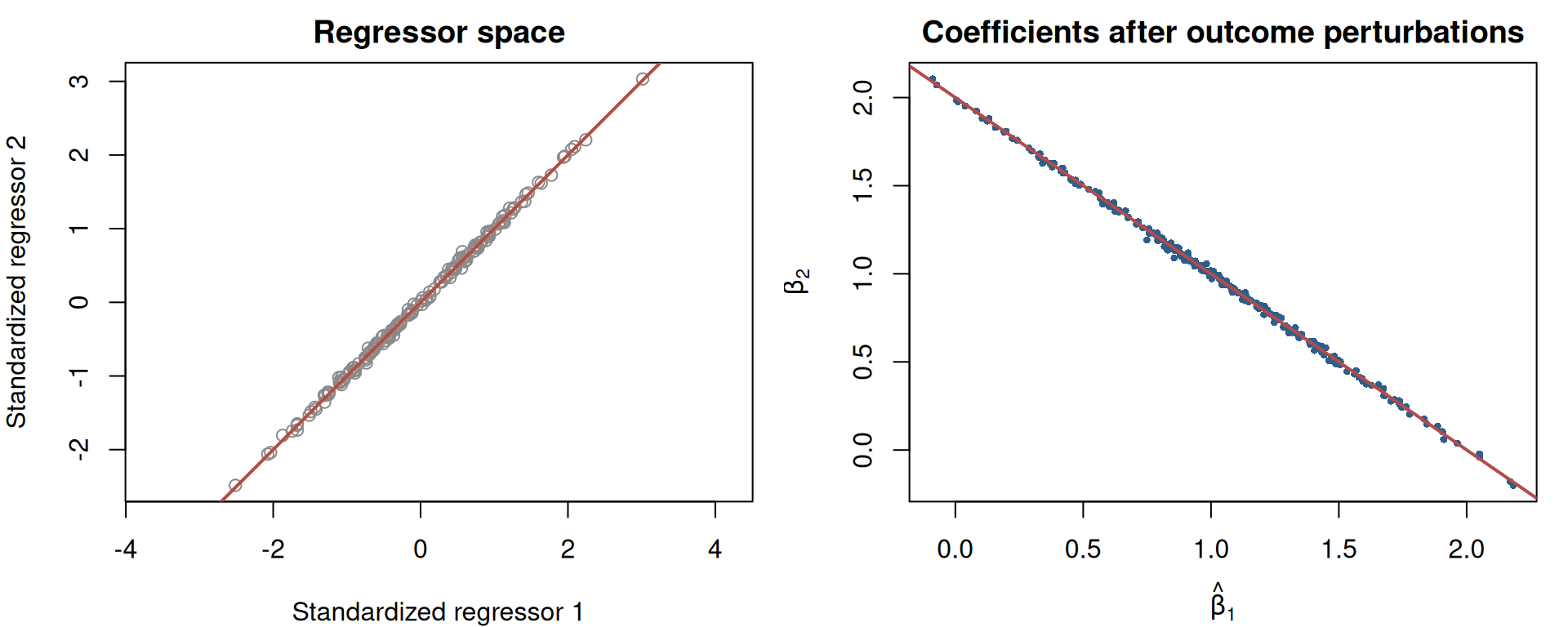
Figure 8 uses two almost identical standardized regressors. Their condition number is approximately 56. Repeated small perturbations of the outcome generate large movements in the individual coefficients. The estimates move in opposite directions, leaving their sum and the fitted values much more stable.
When \(X\) is rank deficient, infinitely many coefficient vectors can produce the same fitted values. The pseudoinverse selects the solution with minimum Euclidean norm. This does not create information in a missing direction; it supplies a well-defined representative among observationally equivalent coefficient vectors. The SVD separates that identification issue from the directions that the data estimate precisely.
Conclusion
The singular value decomposition describes a matrix through matched orthogonal directions. The columns of \(V\) identify input directions, the singular values state how strongly the matrix acts along them, and the columns of \(U\) identify the resulting output directions. The decomposition exists because \(A^\top A\) is a real symmetric positive-semidefinite matrix whose orthonormal eigenvectors provide the required input basis.
For a centered data matrix, the same objects have statistical interpretations. The right singular vectors are principal-component directions, \(UD\) contains observation scores, and squared singular values determine the variance along each component. Retaining the largest singular layers gives the best low-rank approximation. In regression, inverting those layers reveals why weak singular directions produce unstable coefficients. These are different uses of one construction: a matrix becomes transparent once its action is expressed in the directions it treats independently.