Hyperplanes, distances, and margins
Introduction
A linear classifier separates observations by a flat boundary. In two variables the boundary is a line; in three variables it is a plane; and in \(p\) variables it is a hyperplane. Support vector machines use such a boundary, then choose the separating boundary that leaves the largest possible gap between the two classes. The gap is called the margin.
The calculation rests on one fact from Euclidean geometry: the shortest route from a point to a hyperplane follows the vector perpendicular to that hyperplane. This note establishes that fact in coordinates. It then distinguishes an algebraic quantity, the functional margin, from the geometric distance that an SVM maximizes. The optimization problem used to choose the boundary is considered separately.
A hyperplane and its two sides
Let an observation be a column vector \(x\in\mathbb{R}^p\). Let \(w\in\mathbb{R}^p\) be nonzero and let \(b\in\mathbb{R}\) be a scalar. The set
\[ \mathcal H=\{z\in\mathbb{R}^p:w^\top z+b=0\} \]
is an affine hyperplane. The letter \(z\) is used for a generic point on the boundary, reserving \(x\) for the observation whose location is to be assessed. The product \(w^\top z\) is a scalar: \(w^\top\) has dimensions \(1\times p\) and \(z\) has dimensions \(p\times1\). Adding the scalar \(b\) is therefore well defined.
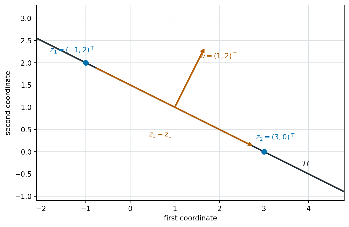
The vector \(w\) is normal, or perpendicular, to \(\mathcal H\). To see this, take any two points \(z_1,z_2\in\mathcal H\). They both satisfy \(w^\top z_j+b=0\), so subtracting their two equations gives
\[ w^\top(z_1-z_2)=0. \]
The difference \(z_1-z_2\) runs along the hyperplane. Its zero inner product with \(w\) shows that every such direction is perpendicular to \(w\). In two dimensions, this says that the line \(w^\top z+b=0\) has normal vector \(w\). Figure Figure 1 gives a two-dimensional example.
The boundary divides the space into two open half-spaces:
\[ w^\top x+b>0 \qquad\text{and}\qquad w^\top x+b<0. \]
The sign determines the side. The intercept \(b\) shifts the boundary away from the origin. When \(b=0\), the boundary passes through the origin and is a linear subspace. When \(b\ne0\), it is affine rather than linear: it remains flat, but no longer contains zero.
The terms linear and affine here have their algebraic meanings.1
Distance from a point to the boundary
For a point \(x\in\mathbb{R}^p\), let \(q\) be its closest point on \(\mathcal H\). The displacement from \(q\) to \(x\) must be perpendicular to the hyperplane, so it must be a multiple of the normal vector. Write
\[ q=x-tw \]
for an unknown scalar \(t\). This expression starts at \(x\) and moves along the normal direction. The sign of \(t\) chooses which of the two directions along that line is used.
Because \(q\) lies on the hyperplane, it satisfies its defining equation. Substitution gives
\[ \begin{aligned} 0 &=w^\top q+b\\ &=w^\top(x-tw)+b\\ &=w^\top x-tw^\top w+b. \end{aligned} \]
The second line substitutes \(q=x-tw\). The last line distributes \(w^\top\) and uses the fact that \(t\) is a scalar. Since \(w\ne0\), \(w^\top w=\lVert w\rVert_2^2>0\), and the equation can be solved for \(t\):
\[ t=\frac{w^\top x+b}{\lVert w\rVert_2^2}. \]
The distance is the length of the displacement \(x-q=tw\), not the value of \(t\) itself. Using homogeneity of the Euclidean norm gives
\[ \begin{aligned} \operatorname{dist}(x,\mathcal H) &=\lVert x-q\rVert_2\\ &=\lVert tw\rVert_2\\ &=|t|\lVert w\rVert_2\\ &=\frac{|w^\top x+b|}{\lVert w\rVert_2}. \end{aligned} \]
This explains the division by \(\lVert w\rVert_2\). The numerator measures position in the arbitrary units of the normal vector \(w\). Multiplying by the length of \(w\) turns the normal-coordinate \(t\) into a Euclidean length, and one factor of \(\lVert w\rVert_2\) remains in the denominator. The signed version retains the side of the boundary:
\[ d_{\mathcal H}(x)=\frac{w^\top x+b}{\lVert w\rVert_2}. \]
It is positive on the side towards which \(w\) points, negative on the other side, and zero precisely on \(\mathcal H\).
The same boundary has many equations
For any positive scalar \(c\), the pairs \((w,b)\) and \((cw,cb)\) describe exactly the same hyperplane, because
\[ cw^\top z+cb=c(w^\top z+b)=0 \quad\Longleftrightarrow\quad w^\top z+b=0. \]
They also assign every point to the same half-space. However, the numerator \(w^\top x+b\) becomes \(c(w^\top x+b)\). It is therefore not a distance. The denominator in \(d_{\mathcal H}(x)\) changes by exactly the same positive factor:
\[ \frac{(cw)^\top x+cb}{\lVert cw\rVert_2} =\frac{c(w^\top x+b)}{c\lVert w\rVert_2} =d_{\mathcal H}(x). \]
Geometric distance is consequently determined by the boundary, whereas the unnormalized expression is not. A negative rescaling describes the same boundary too, but reverses which side is called positive. Classifiers can adopt either orientation provided their class labels are reversed at the same time.
Functional and geometric margins
Suppose a training sample contains \((x_i,y_i)\) for \(i=1,\ldots,n\), where \(x_i\in\mathbb{R}^p\) and \(y_i\in\{-1,+1\}\). The classifier predicts the sign of \(w^\top x_i+b\). Multiplying this score by the observed label yields the functional margin of observation \(i\):
\[ \widetilde\gamma_i=y_i(w^\top x_i+b). \]
This is positive when the observation is on the correctly labelled side of the boundary. For example, when \(y_i=+1\), positivity requires \(w^\top x_i+b>0\). When \(y_i=-1\), positivity requires \(w^\top x_i+b<0\), because multiplication by \(-1\) reverses the sign. The functional margin is negative for a misclassified observation and zero for an observation on the boundary.
The geometric margin divides the functional margin by the normal length:
\[ \gamma_i=\frac{y_i(w^\top x_i+b)}{\lVert w\rVert_2}. \]
Since \(y_i\) is either \(-1\) or \(+1\), its absolute value is one. Thus \(\gamma_i\) is the signed distance from \(x_i\) to the boundary, made positive when the classification is correct. Unlike \(\widetilde\gamma_i\), it does not change if \((w,b)\) is multiplied by a positive constant.
A sample is linearly separable when there are \(w\ne0\) and \(b\) such that
\[ y_i(w^\top x_i+b)>0 \qquad\text{for every }i. \]
In that case every observation is correctly classified and no observation lies on the separating hyperplane. The margin of a given separating boundary is the smallest geometric margin in the sample,
\[ \gamma=\min_{1\leq i\leq n} \frac{y_i(w^\top x_i+b)}{\lVert w\rVert_2}. \]
The minimum matters because the closest observations limit how far the boundary can be moved without reaching one of the classes.
Canonical scaling and support vectors
The rescaling ambiguity can be removed by choosing a convenient normalization. For any separating \((w,b)\), rescale the pair so that the smallest functional margin equals one:
\[ \min_i y_i(w^\top x_i+b)=1. \]
Under this canonical scaling, every observation satisfies
\[ y_i(w^\top x_i+b)\geq1. \]
The observations closest to this particular boundary satisfy equality. They lie on one of two parallel hyperplanes,
\[ w^\top x+b=1 \qquad\text{or}\qquad w^\top x+b=-1, \]
according to their label. Once the max-margin boundary has been chosen, the observations satisfying equality are the support vectors. They support, or pin down, that widest separating gap: moving either parallel boundary inward would meet a support vector first.
With this normalization, the distance from the decision boundary \(w^\top x+b=0\) to either supporting hyperplane is \(1/\lVert w\rVert_2\). This follows directly from the distance formula, since changing the right-hand-side score from \(0\) to \(1\) changes the numerator by one. The total width between the two supporting hyperplanes is therefore
\[ \frac{2}{\lVert w\rVert_2}. \]
Maximizing the margin is consequently equivalent, after imposing the canonical constraints, to minimizing \(\lVert w\rVert_2\) or the equivalent objective \(\tfrac12\lVert w\rVert_2^2\). This converts a geometric aim into the constrained optimization problem used by the hard-margin support vector machine. The remaining step is to solve that problem and to extend it when perfect separation is unavailable.
Conclusion
An affine hyperplane is determined by its normal vector and intercept, but its equation has an arbitrary scale. Dividing the signed score by \(\lVert w\rVert_2\) removes that arbitrariness and yields signed Euclidean distance. Under canonical scaling, the closest correctly classified observations have functional margin one, the two supporting hyperplanes are \(2/\lVert w\rVert_2\) apart, and maximizing their separation becomes minimization of \(\tfrac12\lVert w\rVert_2^2\) subject to classification constraints. Those closest observations are the support vectors that determine the boundary.
Footnotes
Here, linear has its algebraic meaning. A map \(f\) is linear when \(f(c x+d y)=c f(x)+d f(y)\) for every pair of vectors \(x,y\) and scalars \(c,d\); in particular, it satisfies \(f(cx)=cf(x)\). Thus \(x\mapsto w^\top x\) is linear. Adding a nonzero intercept gives the affine map \(x\mapsto w^\top x+b\): generally, \(f(cx)=cw^\top x+b\ne c(w^\top x+b)=cf(x)\). In one dimension, the same distinction is between the linear map \(x\mapsto ax\) and the affine, non-linear map \(g(x)=ax+b\) when \(b\ne0\).↩︎