import numpy as np
import matplotlib.pyplot as plt
from scipy.interpolate import interp1d

def egm_solver(
    beta=0.90,          # Discount factor
    R=1.04,             # Gross interest rate
    gamma=2.5,          # CRRA coefficient
    y_high=10,          # High income
    y_low=5,            # Low income
    pi=0.7,             # Prob(high income)
    a_min=0.0,          # Borrowing constraint (a' >= a_min)
    a_max=20.0,         # Max assets
    n_grid=500,         # Grid size
    tol=1e-8,           # Convergence tolerance
    max_iter=1000       # Max iterations
):
    """
    Solves the consumption-savings problem using the Endogenous Grid Method.
    Budget Constraint: c + a' = R*a + y
    """

    # 1. Setup Grid for a' (Assets tomorrow)
    # We use a' as the exogenous grid for EGM
    a_prime_grid = np.linspace(a_min, a_max, n_grid)

    # Income arrays for vectorized operations
    y_vals = np.array([y_low, y_high])
    # Transition matrix (iid for simplicity based on your code, but expandable)
    # P[i, j] = prob of going from state i to j.
    # Your code implied iid shocks (probs depend only on destination).
    P = np.array([[1-pi, pi],   # From Low
                  [1-pi, pi]])  # From High

    # 2. Initialize Policy Guess (Consumption on the a_prime_grid)
    # Guess: Consume interest + income (stationary)
    # We need two policies: c_low(a) and c_high(a)
    # Initial guess defined on the asset grid
    c_low = y_low + (R - 1) * a_prime_grid
    c_high = y_high + (R - 1) * a_prime_grid

    # Stack for easier matrix math: shape (2, n_grid) -> [Low, High]
    c_policy = np.vstack((c_low, c_high))

    # Pre-calculate Utility Prime helper function
    def marg_util(c):
        return np.maximum(c, 1e-10)**(-gamma)

    for it in range(max_iter):
        c_old = c_policy.copy()

        # --- EGM STEP 1: Expectation ---
        # Calculate Marginal Utility at next period's grid points
        # Since our grid IS a', we don't need to interpolate to find c(a').
        # We use the current guess c_old evaluated at a_prime_grid.
        mu_next = marg_util(c_old) # shape (2, n_grid)

        # Expected Marginal Utility
        # E_mu[0] is E[u'(c')] given we are currently Low income
        # E_mu[1] is E[u'(c')] given we are currently High income
        # Matrix multiplication: (2,2) @ (2, n_grid) -> (2, n_grid)
        E_mu = P @ mu_next

        # --- EGM STEP 2: Invert Euler Equation ---
        # u'(c) = beta * R * E[u'(c')]
        # c = (beta * R * E_mu) ^ (-1/gamma)
        c_endo = (beta * R * E_mu) ** (-1.0 / gamma)

        # --- EGM STEP 3: Endogenous Assets ---
        # Budget: c + a' = R*a + y  =>  a = (c + a' - y) / R
        # We compute the 'a' that would lead to choosing 'a_prime_grid'
        # shape (2, n_grid)
        a_endo = (c_endo + a_prime_grid[None, :] - y_vals[:, None]) / R

        # --- EGM STEP 4: Re-gridding (Interpolation) ---
        # We now have pairs (a_endo, c_endo). We need c on the regular 'a_prime_grid'.
        # We also need to handle the borrowing constraint a' >= a_min.

        c_new = np.zeros_like(c_policy)

        for i in range(2): # Loop over income states (0: Low, 1: High)
            y_curr = y_vals[i]
            a_end_state = a_endo[i, :]
            c_end_state = c_endo[i, :]

            # 4a. Handle the Binding Constraint Region
            # The smallest endogenous asset a_end_state[0] corresponds to a' = a_min.
            # For any a < a_end_state[0], the constraint binds: a' = a_min.
            # Budget when binding: c = R*a + y - a_min

            # We use a custom interpolation wrapper
            def interpolate_policy(a_target, a_end, c_end, y_inc):
                # 1. Linear interpolation for the interior region (a_endo[0] to max)
                c_interp = np.interp(a_target, a_end, c_end)

                # 2. Overwrite the constrained region
                # Where a_target < first endogenous point, the agent wants to borrow more
                # than a_min but can't.
                binding_region = a_target < a_end[0]

                if np.any(binding_region):
                    # c = R*a + y - a_min
                    c_interp[binding_region] = R * a_target[binding_region] + y_inc - a_min

                return c_interp

            c_new[i, :] = interpolate_policy(a_prime_grid, a_end_state, c_end_state, y_curr)

        # Check convergence
        diff = np.max(np.abs(c_new - c_old))
        c_policy = c_new

        if diff < tol:
            print(f"Converged in {it+1} iterations. Diff: {diff:.2e}")
            break

return a_prime_grid, c_policy[1, :], c_policy[0, :]A Reminder of the Endogenous Grid Method
Introduction
The Endogenous Grid Method (EGM) is a numerical technique for solving dynamic stochastic optimization problems, particularly household consumption-savings decisions with constraints. Introduced by Caroll (2006)1, EGM dramatically accelerates computation compared to standard value function iteration (VFI) by exploiting the structure of first-order conditions to construct policy functions directly.
Inverting the Euler Equation
In standard dynamic programming (“exogenous grid method”), we:
- Specify a grid over state variables (e.g., assets a)
- For each grid point, solve an optimization problem to find optimal choices (e.g., consumption c)
- This requires costly numerical maximization at each point
EGM flips this approach:
- Start from the Euler equation (the first-order condition)
- Specify a grid over end-of-period assets (next period’s state)
- Invert the Euler equation analytically to compute current consumption directly
- Derive current assets endogenously from the budget constraint
This eliminates root-finding/maximization at each grid point, yielding 10–100x speed improvements.
Example: Simple Consumption-Savings Problem
Consider a household maximizing expected lifetime utility:
\[\max_{\{c_t\}} \mathbb{E}_0 \sum_{t=0}^{\infty} \beta^t u(c_t)\]
subject to the budget constraint:
\(a_{t+1} = R(a_t + y_t - c_t)\)
where:
- \(a_t\) = assets at beginning of period t
- \(c_t\) = consumption
- \(y_t\) = stochastic labor income (iid)
- \(R = 1+r\) = gross return on assets
- \(\beta\) = discount factor
- \(u(c) = \frac{c^{1-\gamma}}{1-\gamma}\) (CRRA utility)
Standard Approach (Exogenous Grid)
- Create grid \(\{a^1, a^2, ..., a^N\}\) over current assets \(a_t\)
- For each \(a^i\), solve: \(\max_c u(c) + \beta \mathbb{E}[V(a')]\) s.t. \(a' = R(a^i + y - c)\)
- Requires numerical maximization at each grid point
EGM Approach
The Euler equation for this problem is:
\[u'(c_t) = \beta R \mathbb{E}_t[u'(c_{t+1})]\]
The EGM algorithm is as follows:
- Guess next-period policy function \(c'(a')\) (consumption as function of next-period assets)
- Create an exogenous grid over next-period assets: \(\{a'^1, a'^2, ..., a'^N\}\)
- For each \(a'^j\) on this grid:
- Compute expected marginal utility of next period’s consumption: \[\mathbb{E}[u'(c'(a'^j))] = \sum_s \pi_s u'(c'(R(a'^j + y_s)))\] where \(\pi_s\) are income state probabilities
- Invert the Euler equation to get current consumption: \[c^j = (u')^{-1}\left(\beta R \mathbb{E}[u'(c'(a'^j))]\right)\] For CRRA utility: \(c^j = \left[\beta R \mathbb{E}[(c'(a'^j))^{-\gamma}]\right]^{-1/\gamma}\)
- Recover current assets endogenously from budget constraint: \[a^j = \frac{a'^j}{R} + \mathbb{E}[y] - c^j\]
- Construct policy function: You now have pairs \((a^j, c^j)\) defining \(c(a)\). Since \(a^j\) values are irregular (endogenous), interpolate to create a function on a regular grid.
- Iterate until convergence (policy function iteration)
Note that this features no optimization: Step 3 uses analytical inversion instead of numerical maximization , and no root finding: consumption is derived directly from Euler equation. Only interpolation needed at step 4.
Extensions and Applications
EGM has been extended to handle: - Non-convexities (e.g., discrete choices like retirement) via DCEGM (Discrete-Continuous EGM)2 - Borrowing constraints: When \(a_{t+1} \geq \bar{a}\) binds, the Euler equation doesn’t hold; EGM handles this by identifying kink points where constraints bind.3
EGM is now the workhorse method for structural estimation of life-cycle consumption models, precautionary savings models, and heterogeneous agent macro models due to its speed and accuracy.
Implementation in Python
Euler Equation Derivation
For the household problem with CRRA utility \(u(c) = \frac{c^{1-\gamma}}{1-\gamma}\) and iid income \(y_t \in \{y_H, y_L\}\) with probabilities \(\pi\) and \(1-\pi\), the Bellman equation is:
\[V(a, y) = \max_{c} \left\{ u(c) + \beta \mathbb{E}_y \left[ V(a', y') \right] \right\}\]
subject to \(a' = R(a + y - c)\) and \(a' \geq \bar{a}\) (borrowing constraint, typically \(\bar{a}=0\)).
The first-order condition (assuming an interior solution) is:
\(u'(c) = \beta R \mathbb{E}_{y'} \left[ V'_a(a', y') \right]\)
The envelope condition is:
\(V'_a(a, y) = u'(c)\)
Combining these and applying the envelope condition next period (\(V_a(a', y') = u'(c')\)):
\(u'(c_t) = \beta R \mathbb{E}_{y'} \left[ u'(c_{t+1}) \right]\)$
For CRRA utility (\(u'(c) = c^{-\gamma}\)), the Euler equation becomes:
\[c_t^{-\gamma} = \beta R \left[ \pi \cdot c_{t+1,H}^{-\gamma} + (1-\pi) \cdot c_{t+1,L}^{-\gamma} \right]\]
Rearranged for EGM implementation:
\[c_t = \left( \beta R \left[ \pi \cdot c_{t+1,H}^{-\gamma} + (1-\pi) \cdot c_{t+1,L}^{-\gamma} \right] \right)^{-1/\gamma}\]
The Euler equation holds whenever the borrowing constraint is not binding. When the borrowing constraint binds (i.e. \(a_{t+1} = \bar{a}\)) the FOC no longer holds with equality. Instead, consumption is determined by the budget constraint: \(c_t = a_t + y_t - \frac{\bar{a}}{R}\).
In EGM, we detect binding constraints by checking whether the endogenously recovered \(a_t\) falls below \(\bar{a}\) and adjust consumption accordingly (as shown in the Python code).
Efficient Python Implementation of EGM
This implementation solves the aforementioned consumption-savings problem with:
- Two income states (\(y_H\), \(y_L\)) with probabilities \(\pi\) and \(1-\pi\) respectively.
- Borrowing constraint \(a' \geq 0\)
- Policy function iteration with EGM
- Vectorized operations for speed
Example Usage and Visualization
# Solve the model
beta=0.90 # Discount factor
R=1.04 # Gross interest rate
gamma=2.5 # CRRA coefficient
y_high = 3.0 # High income
y_low = 1.0 # Low income
pi=0.7 # Probability of High
a_grid, c_high, c_low = egm_solver(
beta=beta,
gamma=gamma,
y_high = y_high,
y_low = y_low,
R = R,
pi = pi,
a_max=20
)
plt.figure(figsize=(10, 6))
plt.plot(a_grid, c_high, label='High Income', linewidth=2)
plt.plot(a_grid, c_low, label='Low Income', linewidth=2)
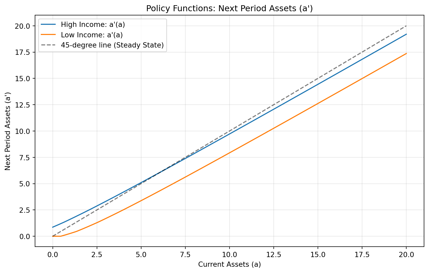
# Plot the 45-degree line-like concept (Asset accumulation)
# a' = R*a + y - c. Let's plot a' (savings)
a_prime_high = R * a_grid + y_high - c_high
a_prime_low = R * a_grid + y_low - c_low
plt.figure(figsize=(10, 6))
plt.title("Policy Functions: Next Period Assets (a')")
plt.plot(a_grid, a_prime_high, label="High Income: a'(a)")
plt.plot(a_grid, a_prime_low, label="Low Income: a'(a)")
plt.plot(a_grid, a_grid, 'k--', alpha=0.5, label="45-degree line (Steady State)")
plt.xlabel("Current Assets (a)")
plt.ylabel("Next Period Assets (a')")
plt.legend()
plt.grid(True, alpha=0.3)
plt.show()Converged in 82 iterations. Diff: 9.26e-09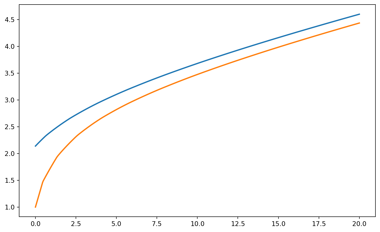
Summary
In this blog, we have implemented a true EGM approach. An exogenous grid on \(a'\) (next-period assets), using the Euler equation inverted analytically to get \(c\) directly, and recovered current assets \(a\) recovered endogenously via \(a = a'/R + y - c\). We also handled binding constraints, our function detects when \(a < a_{\min}\) (borrowing constraint binds), and adjusts consumption to satisfy \(a' = a_{\min}\) exactly.