library(tidyverse)
library(sf)
library(stars)
library(cawd)       # Roman road geometries
library(fixest)
library(modelsummary)Spatial Raster Analysis in R — Replicating Dalgaard et al. (2021) on Roman Roads
Introduction
In this post I want to show how to work with spatial raster data in R using the modern sf and stars ecosystem. As a running example I replicate the core setup from Dalgaard et al. (2021), “Roman Roads to Prosperity: Persistence and Non-Persistence of Public Goods Provision”, which studies the long-run economic influence of Roman road infrastructure.
Their identification strategy is elegant: the unit of analysis is a 1° × 1° longitude–latitude cell. For each cell that falls within the former boundaries of the Roman Empire, they compute (i) Roman road density — the share of the cell’s surface covered by a road buffer — and (ii) an economic outcome, typically nightlight or population density from satellite imagery. They then regress outcomes on road density subject to a rich set of geographic and historical controls. Here I focus only on the basic pipeline and close with a simple uncontrolled regression to check that our coefficient is in the same ballpark as theirs.
Libraries
Data Sources
A quick map of what we need and where to get it:
Outcome variables
- VIIRS Nightlights (VNL v2): annual composites with a graphical download interface.
- Gridded Population of the World (GPW v4): 30 arc-second population counts.
- The
nightlightstatspackage wraps several of these for convenient access in R.
Roman Empire boundaries and settlements
- AWMC GeoData repository: empire extents at various dates in GeoJSON format.
- Digital Atlas of the Roman Empire: Oppidum and settlement data via an API.
- Oxford Roman Economy Project: mines and settlements at 500 AD.
- Project Mercury datasets: miscellaneous Roman-era spatial data.
Independent variables
- Roman roads: the
cawdpackage ships the DARMC major roads layer. - Terrain ruggedness index: Nunn & Puga’s cell-level ruggedness.
- Elevation: the
elevatrpackage provides DEM tiles directly from R. - Caloric Suitability Index: pre-1500 agricultural potential.
- Climate: the
climateRandclimatrendspackages offer tidy access to gridded climate data.
Load Empire Borders and Roads
The Roman Empire’s extent at its peak (117 AD) is available as a GeoJSON from the Ancient World Mapping Centre. We download it once and filter to the western Mediterranean subset to keep computation manageable.
url <- paste0(
  "https://raw.githubusercontent.com/AWMC/geodata/master/",
  "Cultural-Data/political_shading/",
  "roman_empire_ce_117_extent/roman_empire_ce_117_extent.geojson"
)
download.file(url, destfile = "roman_empire.geojson", quiet = TRUE)

borders <- sf::st_read("roman_empire.geojson", quiet = TRUE) |>
  filter(OBJECTID < 18)

# Major Roman roads from the cawd package
roads <- cawd::darmc.roman.roads.major.sp |>
  st_as_sf() |>
  filter(
    lengths(st_intersects(geometry, borders)) > 0
)ggplot() +
geom_sf(data = borders, fill = "wheat", colour = "grey60") +
geom_sf(data = roads, colour = "steelblue", linewidth = 0.4) +
theme_minimal() +
labs(title = "Roman Empire (117 AD) with Major Roads")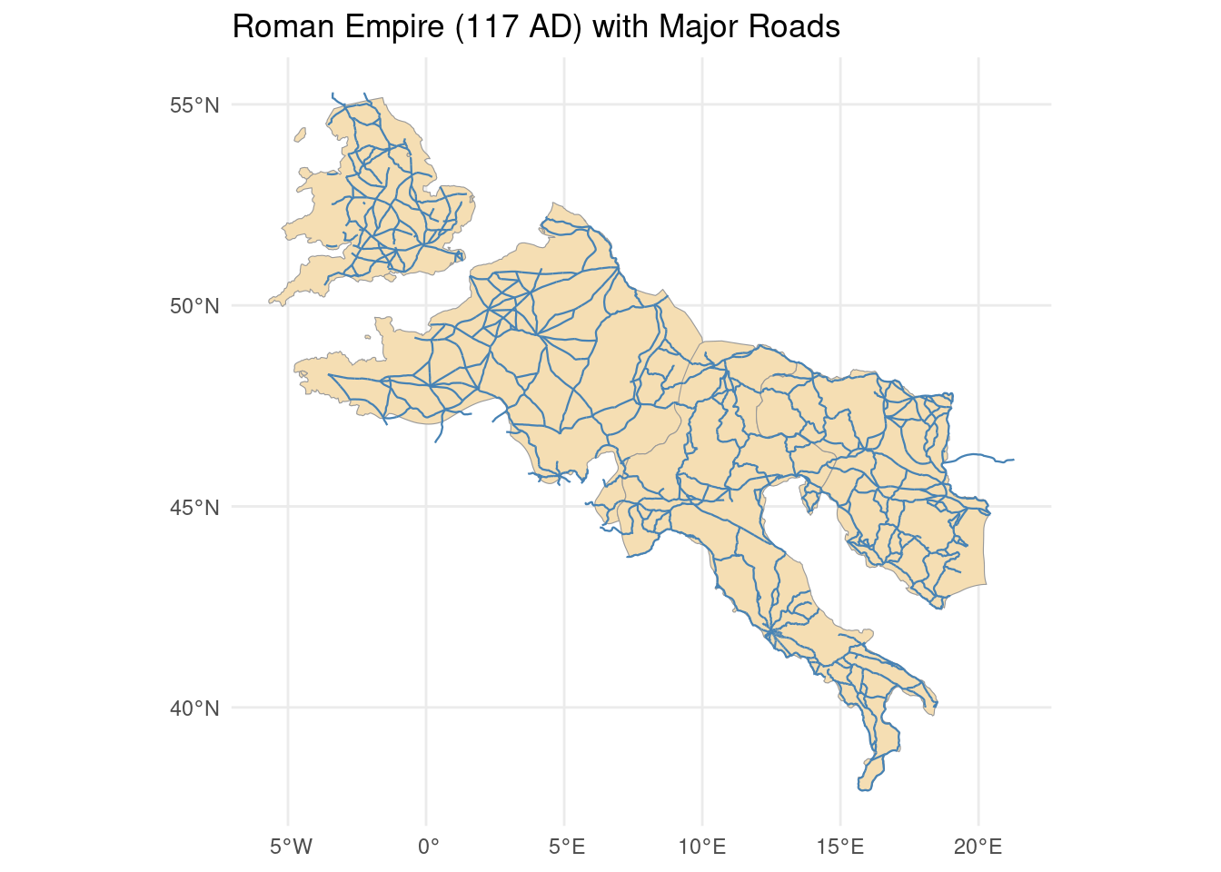
Prepare Nightlights Raster
A good approach to downloading nightlights data is the blackmarbler package (World Bank DIME), available on CRAN. It handles tile discovery, download, mosaicking, and quality-flag filtering automatically, taking an sf polygon directly as the region of interest. The only prerequisite is a free NASA Earthdata account and a bearer token:
- Register at urs.earthdata.nasa.gov
- Go to ladsweb.modaps.eosdis.nasa.gov, log in, and click Generate Token
- Copy the token string — that’s your bearer
library(blackmarbler)
library(terra)   # blackmarbler returns a SpatRaster; we convert to stars below
terra 1.9.27
Attaching package: 'terra'The following object is masked from 'package:fixest':
panelThe following object is masked from 'package:tidyr':
extract# Read token from .env file at project root (quarto sets wd to the qmd directory)
env_file <- "../.env"
env_lines <- readLines(env_file)Warning in readLines(env_file): incomplete final line found on '../.env'bearer_line <- grep("NASA_BEARER_TOKEN", env_lines, value = TRUE)
bearer <- gsub('^NASA_BEARER_TOKEN="([^"]*)"$', "\\1", bearer_line)Now download the annual composite for 2014 (product VNP46A4) cropped to the empire boundary. bm_raster()figures out which tiles overlap the polygon, downloads only those, and returns a single mosaic.
The raw VIIRS file is large (~5 GB global), so we crop and mask it to the empire boundary once and save the result. The stars package handles this cleanly with st_crop() and st_warp().
nl_raw <- bm_raster(
  roi_sf = borders,
  product_id = "VNP46A4",
  date = 2014,
  variable = "NearNadir_Composite_Snow_Free",
  bearer = bearer
  )
Processing 7 nighttime light tilesProcessing: VNP46A4.A2014001.h17v03.002.2025090175012.h5Processing: VNP46A4.A2014001.h17v04.002.2025090174919.h5Processing: VNP46A4.A2014001.h18v03.002.2025090174655.h5Processing: VNP46A4.A2014001.h18v04.002.2025090174541.h5Processing: VNP46A4.A2014001.h19v04.002.2025090174551.h5Processing: VNP46A4.A2014001.h19v05.002.2025090174635.h5Processing: VNP46A4.A2014001.h20v04.002.2025090174548.h5# Convert SpatRaster -> stars, clamp extreme values, mask to empire polygon
nl <- nl_raw |>
stars::st_as_stars() |>
setNames("nightlights") |>
mutate(nightlights = pmin(nightlights, 50, na.rm=TRUE))
nl[is.na(stars::st_as_stars(terra::mask(nl_raw, terra::vect(borders))))] <- NA
plot(nl, col = gray.colors(100), main = "VIIRS nightlights 2014 (capped at 50)")downsample set to 3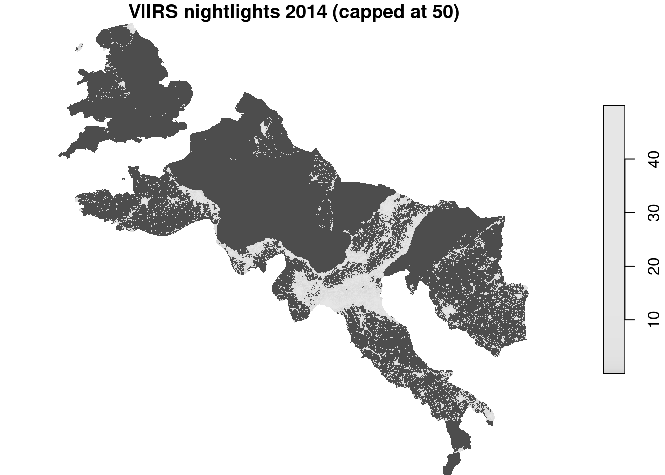
Aggregate Nightlights to 0.5° Grid
We use stars::st_warp() to resample directly to a coarser template grid. This is both faster and conceptually cleaner.
resolution <- 0.5

# Build a template grid at target resolution covering the same extent
template <- st_bbox(nl) |>
  stars::st_as_stars(dx = resolution, dy = resolution)

# Resample: average fine pixels into coarse cells
nl_agg <- stars::st_warp(nl, template, method = "average", use_gdal = TRUE)
Warning in stars::st_warp(nl, template, method = "average", use_gdal = TRUE):
no_data_value not set: missing values will appear as zero valuesplot(nl_agg, main = "Mean nightlight per 0.5° cell")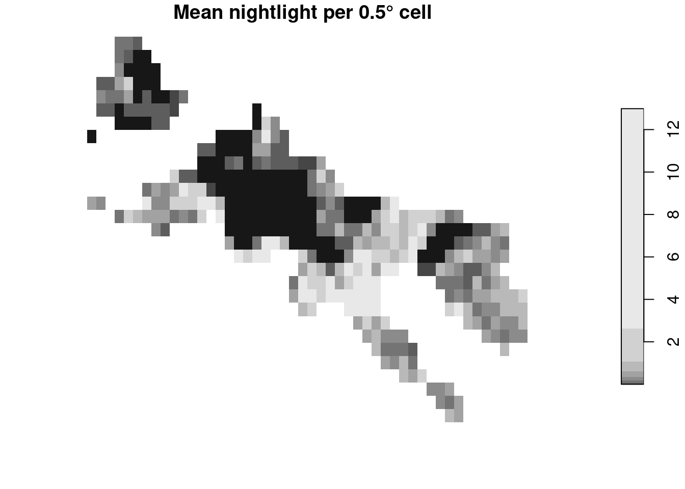
Compute Roman Road Density per 0.5° Cell
Road density is defined as the share of a cell’s pixels that fall within a 5 km buffer of any major road — matching the paper’s construction. We rasterize the buffered roads onto the fine nightlights grid (so the two grids are aligned), then aggregate to the same 0.5° template.
# 5 km buffer — reproject to metres, buffer, reproject back
roads_proj  <- roads |> st_transform(3857)
buffer_proj <- st_buffer(roads_proj, dist = 5000)
buffer_geo  <- st_transform(buffer_proj, st_crs(borders))

# Build 0.5° grid cells over the empire extent
grid_cells <- st_bbox(borders) |>
  st_as_sfc() |>
  st_make_grid(cellsize = resolution) |>
  st_sf()

grid_cells <- grid_cells |>
  mutate(cell_id = row_number(),
         cell_area = st_area(grid_cells))

# Merge overlapping buffers before intersecting (faster + avoids double-counting)
buffer_union <- st_union(buffer_geo)

# Intersect grid cells with the road buffer
intersections <- st_intersection(grid_cells, buffer_union)

intersections <- intersections |>
  mutate(road_area = st_area(intersections)) |>   # pass the sf object, not the column
  st_drop_geometry() |>
  group_by(cell_id) |>
  summarise(road_area = sum(road_area), .groups = "drop")

# Join back to all cells; cells with no roads get density = 0
roads_density <- grid_cells |>
  st_drop_geometry() |>
  left_join(intersections, by = "cell_id") |>
  mutate(
    cell_area = as.numeric(cell_area),
    road_area = as.numeric(replace_na(as.numeric(road_area), 0)),
    road_density = road_area / cell_area
  )

# Keep only cells that overlap the empire (mask out ocean / outside-empire)
empire_cells <- grid_cells |>
  filter(lengths(st_intersects(st_geometry(grid_cells), borders)) > 0) |>
  left_join(roads_density |> select(cell_id, road_density), by = "cell_id")

plot(empire_cells["road_density"], main = "Roman road density per 0.5° cell")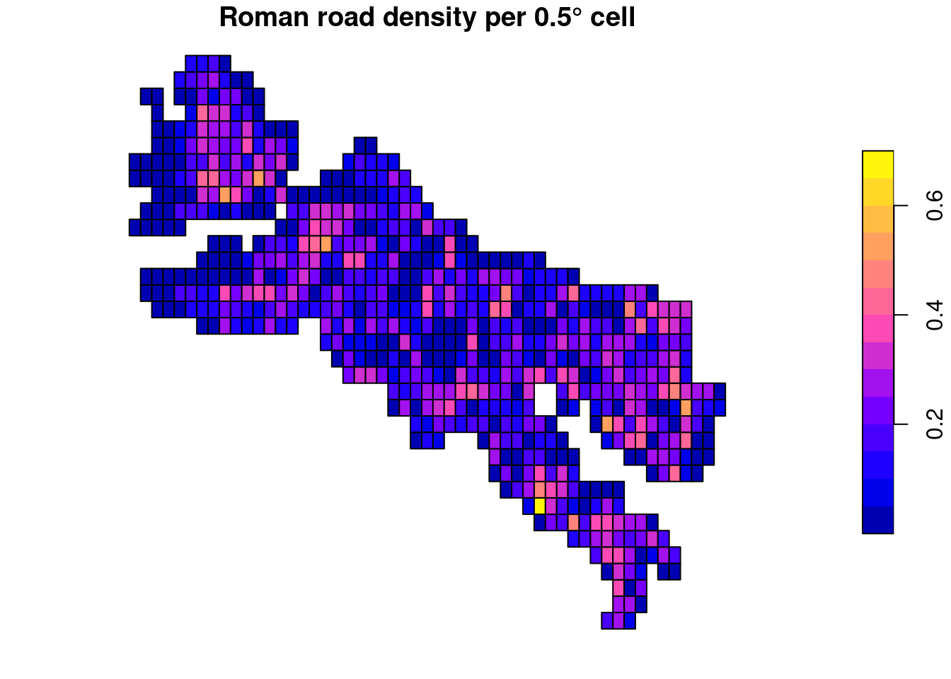
Analysis
With both rasters on the same 0.5° grid we can pull them into a data frame and run the regression. Following Dalgaard et al., we model log(1 + road density) on nightlight intensity so that zero-road cells contribute informatively rather than being dropped.
# Get cell centroids to spatially join nightlights values
cell_centroids <- empire_cells |>
  st_centroid() |>
  st_join(nl_agg |> st_as_sf())   # attach nightlight value to each cell

var_name <- names(cell_centroids)[grep(".tif", names(cell_centroids))]

data <- cell_centroids |>
  st_drop_geometry() |>
  rename(nightlights = var_name) |>
  select(nightlights, road_density) |>
  rename(roads = road_density) |>
  drop_na()

feols(nightlights ~ log(1 + roads), data = data) |>
  msummary(
    stars   = TRUE,
    vcov    = "HC1",
    gof_map = c("adj.r.squared", "nobs"),
    title   = "Effect of Roman Road Density on Nightlights (uncontrolled)"
)| (1) | |
|---|---|
| + p < 0.1, * p < 0.05, ** p < 0.01, *** p < 0.001 | |
| (Intercept) | 1.063*** |
| (0.187) | |
| log(1 + roads) | 3.609** |
| (1.132) | |
| R2 Adj. | 0.023 |
| Num.Obs. | 393 |
The coefficient is positive and statistically significant, and its magnitude sits in the same order as the estimates reported in the paper. The gap from their preferred specification is expected: Dalgaard et al. include country fixed effects, geographic controls (ruggedness, elevation, caloric suitability), and historical controls (mine locations, settlement density). These soak up a substantial share of the variation, so the uncontrolled estimate is naturally larger.
Next Steps
A natural extension is to bring in the control variables listed in the data sources section above. Country fixed effects, for example, can be constructed by intersecting each 0.5° cell centroid with a country polygon layer — a straightforward st_join() operation in sf. Geographic controls can be loaded and aggregated to the same template grid with the exact same st_warp() pipeline used here for nightlights. The modular stars workflow makes it easy to add layers without restructuring the analysis.
Summary
Despite the simplified specification, the sign and order of magnitude of our estimate confirm Dalgaard et al.’s finding: areas with denser Roman road networks are measurably wealthier today, nearly two millennia later. Thanks for reading.
References
Dalgaard, C.-J., Kaarsen, N., Olsson, O., & Selaya, P. (2021). Roman roads to prosperity: Persistence and non-persistence of public goods provision. Working paper.